Data Processing
One of the challenges associated with remote sensing data is the processing steps a user must go through in order to make the data analysis-ready. Radar data, specifically the side-looking characteristic of its data collection mechanism, presents its own specific set of processing challenges. Let’s explore those challenges and required corrective steps here.
Data Distortion
The data values collected by SAR systems can be distorted in two primary ways: geometric and radiometric.
Geometric
Slant range. This type of distortion is caused by the fact that the distance between the radar antenna and the target, known as the slant range, is not constant along the image. This happens because the radar antenna is not perpendicular to the ground, but rather it is pointed at an angle (side-looking). Thus, within a radar image, objects that are closer to the radar system appear compressed while objects farther away are more stretched out. The image does not represent the true horizontal, ground range distance on the surface of the Earth. In order to measure distances between objects, this distortion must be corrected.
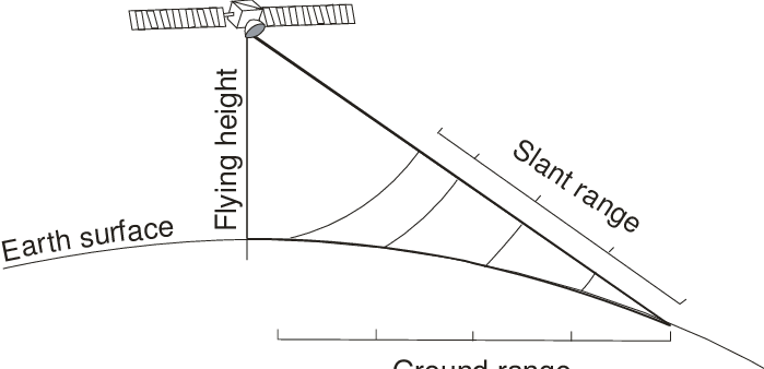
Slant range vs ground range. Source: Tiago Silva, Quantifying Antarctic Icebergs and their Melting in the Ocean.
Layover. This type of distortion occurs more often in mountainous areas. This error will cause features to appear at the wrong location or in the wrong direction because of the timing in which the radar beam hits the object. For example, a radar beam may hit the top of a tall mountain before it hits the base of the mountain. Since it reached the top of the mountain first, it will receive the signal from the top of the mountain earlier than the signal from the base of the mountain, and will thus appear shifted towards the radar system and look as though the top of the mountain is laid over the base.
Foreshortening. This type of distortion occurs when an object is tilted towards the radar system, as in mountainous areas. The angle between the base and the top of the object will appear compressed due to the timing in which the radar beam hits the object and the fact that radars have slant range distortions. Foreshortening severity can vary, and is most severe when the radar beam is directly perpendicular to the object’s slope. For example, if a radar beam hits the base of a mountain before it hits the top of the mountain, the distance between the base and the top of the mountain will appear much shorter than the actual physical distance because of slant range distortions.
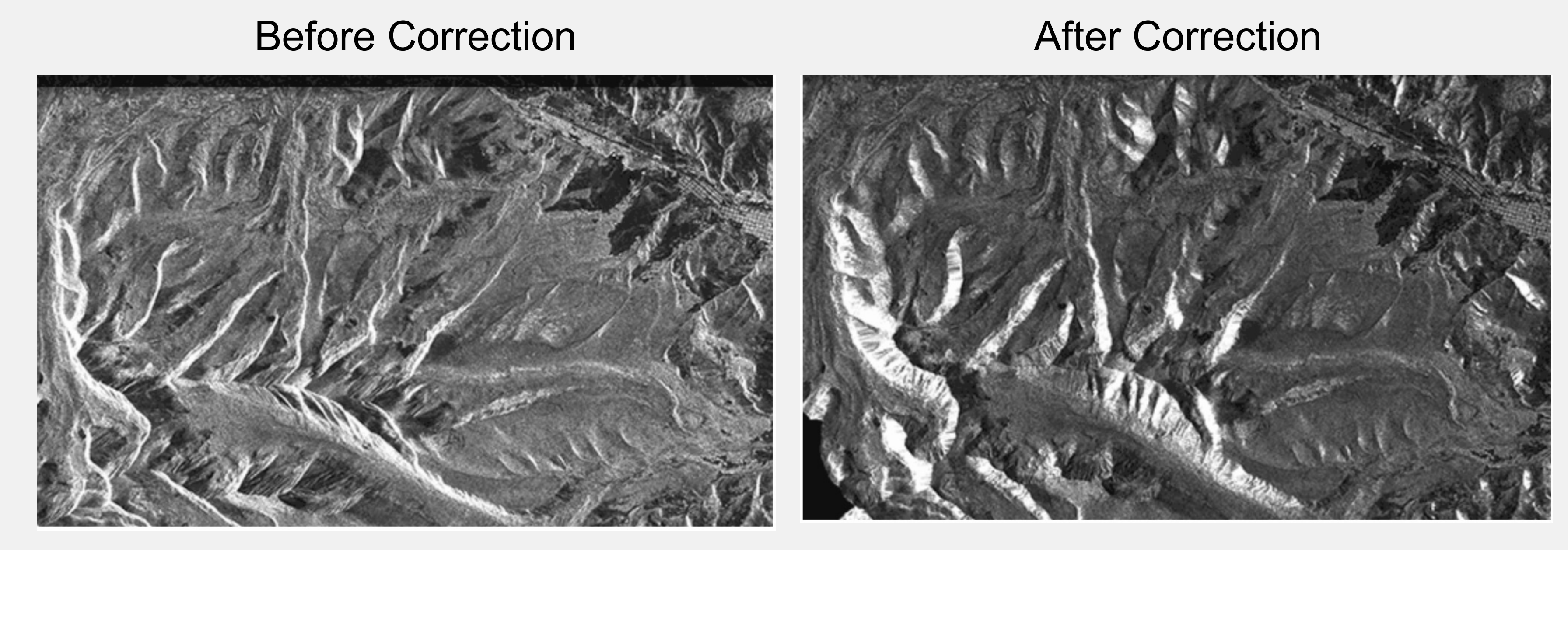 Foreshortening before (left) and after (right) correction. Source: NASA Applied Remote Sensing Training Program
Radiometric
Antennae pattern and signal strength. Radar beams emit more power in the middle of the swath rather than the near or far portions of the swath. This results in an image that has stronger results in the center rather than the near or far edges. This distortion is called the antennae pattern, and it varies significantly depending on the range of the image. Across an image swath, the strength of the return signal diminishes in the farther ranges of the swath. Part of the antennae correction may include a step to produce a uniform average brightness to correct for this effect.
Topographic effects. Topography, especially complex topography, may skew the backscatter values received by the radar system. Steep slopes can, for instance, cause a brightening effect. These effects must be removed in order to capture data related to the characteristics of the Earth you are interested in studying, such as vegetation or soil moisture.
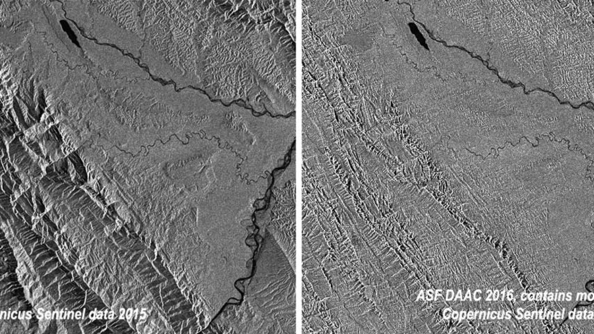 Radiometric correction: before (left) and after (right). Source: Alaska Satellite Facility
Additional Challenges
Shadow. This type of error is conceptually similar to that of clouds in optical imagery. When the radar beam illuminates a large or steep vertical object, such as a mountain or tall building, it may be unable to illuminate the ground on the farther side of the object, resulting in shadow effects on the image. The effect is particularly pronounced at the top of the vertical object, where the incidence angle is larger. Although you can apply some shadow corrections and attempt to fill in the data gaps using interpolation methods, many researchers choose to treat the shadows as missing data – just like the masked out portions of cloudy images.
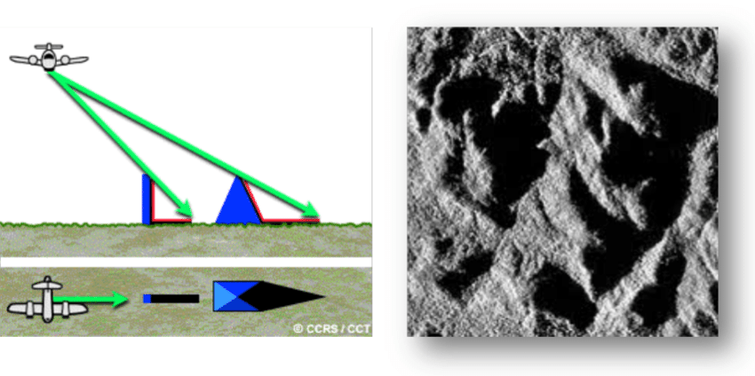
Shadow in SAR imagery. Source: Jolanda Patruno, Polarimetric RADARSAT-2 and ALOS PALSAR multi-frequency analysis over the archaeological site of Gebel Barkal (Sudan).
Speckle. This error is the result of random noise and interference from the radar waves that occurs within the pixel cell. It results in a grainy, almost salt-and-pepper image appearance. There are lots of different gray tones that may appear within a single, uniform surface as the result of speckling. These variations must be filtered in order to improve the visual quality of the data and make it easier to identify features. Unfortunately, the correction method often used to reduce speckling reduces the resolution, so you must balance the visual quality of the image with the resolution of data.
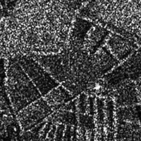
Speckle in SAR imagery. Source: Natural Resources Canada
Data Correction
Given these data distortions, how do we go about correcting them? There are a number of techniques a scientist can use to correct SAR data. In this section, we will be working with a Sentinel-1 C-band SAR image in the state of Amapá, Brazil for the date January 20, 2023. Note that the data we are using is of the product type GRD, or “ground range detected.” That means that the slant range geometric correction has already been performed by the data provider. You should use these types of images when you can to minimize the number of corrective steps you must perform.
Data Preprocessing with SNAP
The European Space Agency (ESA) developed a Sentinel-1 toolbox that you can download and use to process and analyze radar images on their free, open-source software called the Sentinel Application Platform (SNAP). This toolbox allows users to perform, among other processes:
- Calibration
- Speckle noise filtering
- Terrain correction
- Mosaic production
- Classification
Exercise 2.1 Opening and Viewing SAR imagery in SNAP.
Open the SNAP software.
- Click
File > Open Product… - Navigate to the
intro-radar-datafolder on your computer and select the fileS1A_IW_GRDH_1SDV_20230120T090602_20230120T090627_046865_059EA0_7322.zip. Do not unzip this file – SNAP will do it for you! - Click
Opento bring in the image file. You should now see the image listed in theProduct Explorerpanel. - Click on the
+next to the filename to look inside the file. You should see five directories listed:Metadata: Contains detailed information about the image file, including polarization, latitude and longitude, paths, resolution, etc.Vector DataTie-Point Grids: Includes interpolation of latitude and longitude, incidence angle, etc.QuicklooksBands: The actual image data used to conduct data analysis. Contains theAmplitudeandIntensity(which is amplitude squared).
- Click on the
+next to theBandsdirectory. Now, double-click on the band namedAmplitude_VV. - You can click on the
World Viewtab in the lower left-hand panel to see a true-color visualization of the image you are looking at. Drag the globe and zoom in to the red square (the footprint of the image) to take a look. Notice that the image in your image viewer appears mirrored compared to the true color image on the globe – it appears inverted because it is oriented the same way it was acquired. - View RGB image. Right-click on the file name in the
Product Explorerpanel. Select theOpen RGB Image Windowoption. Leave the default options and clickOK. - Inspect pixel values. Return to the original
Amplitude_VVimage. Click on thePixel Infopanel tab next to theProduct Explorerpanel. Move your cursor around the image – you can see information such as the longitude, latitude, amplitude, and intensity automatically show up in the window.
Well done! You have opened, viewed, and inspected a SAR image. But we can’t perform any analysis just yet – as you may have noticed, this image appears quite speckled and we haven’t performed all the required radiometric or geometric correction steps. Our current image is quite large, however, so we first need to take a subset of the image to perform the methods on to ensure the processing goes smoothly.
Exercise 2.2 Pre-process SAR imagery.
- Create an image subset.
- In the upper menu bar, select
Raster > Subset…. - Set the following parameters:
- Scene start X:
8775 - Scene start Y:
2230 - Scene end X:
23315 - Scene end Y:
14930
- Scene start X:
- Click
OK.
- In the upper menu bar, select
- Return to the
Product Explorerpanel. You should see a new file listed that looks likesubset_0_of_[FILE NAME]. Click on the+next to the file, expand theBandsfolder, and double-click onAmplitude_VVto add the subset to the image viewer. Feel free to close the previous images we opened in the viewer to keep things organized. - Perform radiometric calibration.
- Click on the
subsetfilename in theProduct Explorerwindow to highlight the file. - In the upper menu bar, select
Radar > Radiometric > Calibrate. - Leave all of the default options as is, except for the directory. Set the directory as your
intro-radar-datafolder. - Click
Run. It may take a few seconds for the calibration to complete depending on the speed of your computer. - Once the process has completed, click
Close. You should see a new file listed under theProduct Explorerwindow – this is the calibrated image. - Add the
Sigma0_VVband to the image viewer. This image should appear somewhat darker, as there have been multiple corrections made due to antennae pattern, signal strength, saturation, etc.
- Click on the
- Reduce speckle. To filter out the image speckling, we will use a technique called multilook. Multilook divides the radar beam into a number of “sub-beams”, each of which are a single “look” at the scene. The “looks” are summed and averaged together which will reduce the amount of speckle in the final image.
- In the upper menu bar, go to
Radar > SAR Utilities > Multilooking. - In the pop-up window, click on the
Processing Parameterstab. Set theNumber of Range Looksto6. Make sure the directory is set to yourintro-radar-datafolder. - Click
Run. - Click
Close. Another new file should appear in theProduct Explorerwindow. - Add the
Sigma0_VVband to the image viewer. There is a big improvement between the original image and the new image!
- In the upper menu bar, go to
- Perform geometric calibration. Although these images have already been adjusted to ground range rather than slant range, we still need to adjust for any displacement due to terrain.
- In the upper menu bar, go to
Radar > Geometric > Terrain Correction > Range-Doppler Terrain Correction. - Note that this process relies on a digital elevation model (DEM) to make the corrections. You may customize the DEM by clicking on the
Processing Parametersand selecting any of the options in theDigital Elevation Modeldrop-down menu, or using your own if you have one. We will be sticking with the default options for this exercise. - Click
Run. This process may take quite a few seconds to complete. - Click
Close. - Add the
Sigma0_VVband to the image viewer. You should now see a mirror image that looks more in line with the true color image in theWorld Viewer.
- In the upper menu bar, go to
- Convert sigma0 to dB. Backscatter is conventionally represented in the units
dB, which is a representation of the power of the signal.- Right-click on the
Sigma0_VHband of the most recently corrected version of our image. - Select the
Linear to/from dBoption. - In the pop-up window, select
Yes. - Repeat steps a-c for the
Sigma0_VVband. - Add both of the
dbbands to the image viewer and inspect the data.
- Right-click on the
Nice work! You have now successfully pre-processed a radar image and made it ready for data analysis. Notice what a difference the correction steps made from the original downloaded image to the analysis-ready image.