Part 1 - Gathering Data

Overview

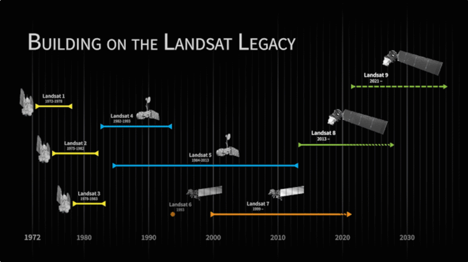
In this workflow, we will create an archive of Landsat imagery from Landsat missions 5 through 9, filter the image archive down to a desired time period of interest, add elevation and Synthetic Aperture Radar (SAR) data (from Copernicus), and then use the data to classify mangrove presence using a Random Forest classification model.

Follow along by copying and pasting each code block in the lesson into your own blank script. At the end you will have the entire workflow saved to a script file on your own GEE account.

Setting up Area of Interest

An area of interest can be uploaded from a local shapefile, drawn on the map, or derived from a pre-existing dataset in the Earth Engine catalogue.

As an example, we will look at the Food and Agriculture Organization’s Global Administrative Units Layer (FAO GAUL) dataset. At the top of the code editor, type in the search bar ‘FAO GAUL Global First’. We see that it is a FeatureCollection containing Level 1 administrative boundaries globally.

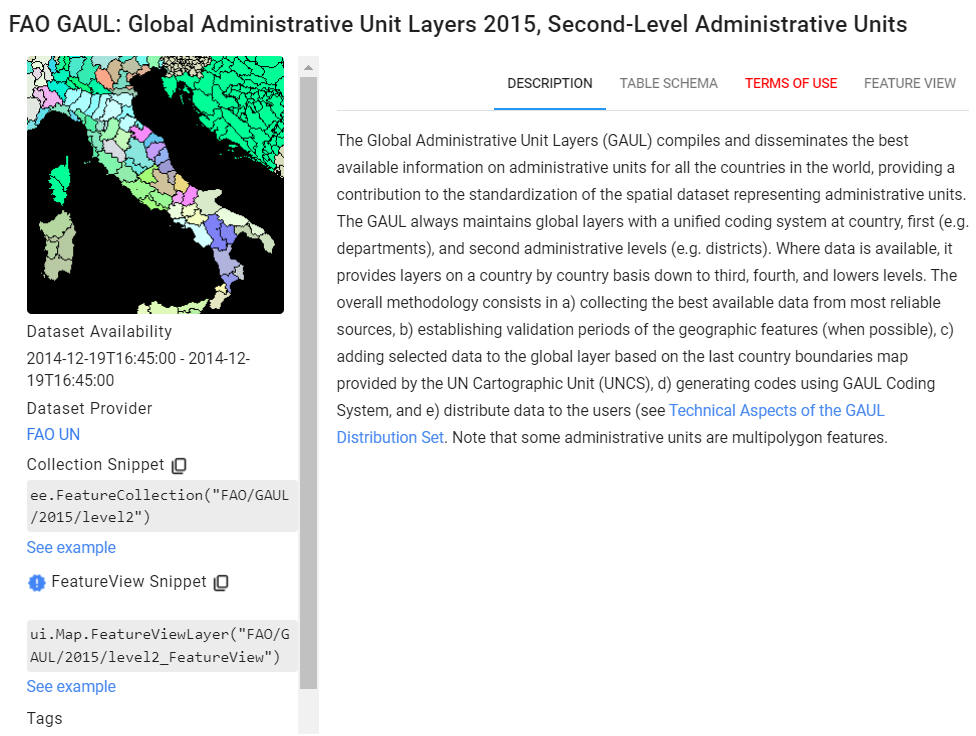
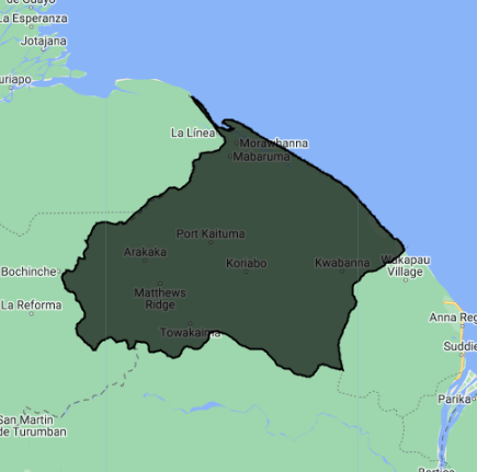
Click on the Table Schema tab. We notice there is a useful field named ‘ADM1_CODE’. We will use this property to derive our AOI. We will focus in on the Barima Waini area and the mangrove area on its coast. Once you add the FAO GAUL data set to the map, you can find the ‘ADM1_CODE’ for this region by clicking on the map while in Inspector mode, and navigating to Objects > FAO Boundaries > 0 > properties.

///--------------------------------------------------------------
// Define vector data (area of interest, aoi)
//--------------------------------------------------------------

// Define an aoi by filtering the FAO GAUL dataset
// https://developers.google.com/earth-engine/datasets/catalog/FAO_GAUL_2015_level1
var boundaries = ee.FeatureCollection("FAO/GAUL/2015/level1");
Map.addLayer(boundaries, {}, 'FAO boundaries');
var aoi = boundaries.filter(ee.Filter.eq('ADM1_CODE', 1398));

// Center the Map on the aoi object, with a specified zoom-level 
// (between 1-24)
Map.centerObject(aoi, 7);

// // Add the aoi object as a layer to the map
Map.addLayer(aoi, {}, 'AOI');

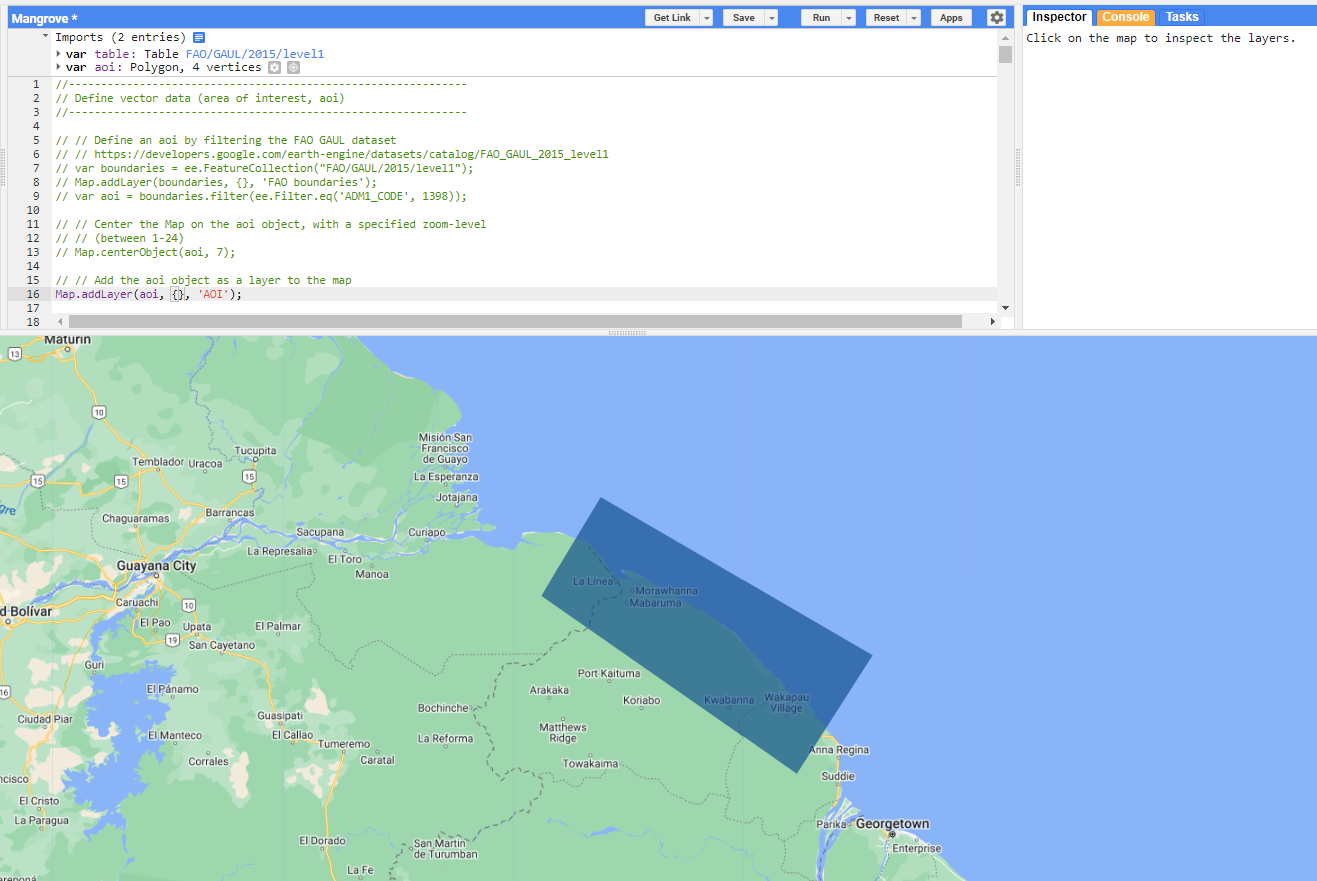
However, for this section, we will create an AOI by drawing a polygon. Comment out all the code above, and utilize the geometry drawing tools in the Map window to draw an area of interest. In the top-left of the Map window, select the Polygon draw button, then create your polygon over the coast in this region. At the top of your script, rename it from ‘geometry’ to ‘aoi’.

Preprocessing Image Collections

First, let’s import our elevation and SAR data. We will use a Digital Elevation Model (DEM) produced from Copernicus data with a 30m resoltuion, and we will use SAR from Copernicus with a 10m resolution. For the SAR data, we will filter for the dates we want, create a median composite, sepcify a couple other parameters, and apply a focal mean filter to reduce speckling (which is a common artifact of SAR).

//--------------------------------------------------------------
// Define raster data (Landsat, Copernicus SAR, Copernicus DEM)
//--------------------------------------------------------------

// Copernicus DEM ----------------------------------------------

// import the DEM band from the Copernicus DEM data set
var demCollection = ee.ImageCollection('COPERNICUS/DEM/GLO30');
var elevation = demCollection
    .select('DEM')
    .mosaic()
    .clip(aoi);
var elevationVis = {
  min: 0.0,
  max: 50,
  palette: ['0000ff','00ffff','ffff00','ff0000','ffffff'],
};

// add DEM to the map
Map.addLayer(elevation, elevationVis, 'DEM');

// Copernicus SAR ----------------------------------------------

// import the VV and VH bands from the Copernicus SAR imagery 
var SARcollection = ee.ImageCollection('COPERNICUS/S1_GRD') 
.filter(ee.Filter.eq('instrumentMode', 'IW'))
// .filter(ee.Filter.eq('orbitProperties_pass', 'ASCENDING'))
// .filterMetadata('resolution_meters','equals',10)
.filterBounds(aoi)
.select('VV','VH')

// filter for the year we want
var SAR = SARcollection.filterDate('2020-01-01','2023-01-01').median().clip(aoi);

// define visualization parameters
var SARvis = {bands:['VV'],min:-20,max:0};

// apply speckle filter
var smoothingRadius = 50;
var SARFiltered = SAR.focal_mean(smoothingRadius,'circle','meters');

// add filtered SAR to map
Map.addLayer(SARFiltered, SARvis,'SAR',false);

We always want to apply filters to ImageCollections as early in our workflow as we can to reduce the amount of effort the GEE servers will require. We already know the area that we’d like to pull data for (our AOI), and that we want relatively few clouds in our images, so we will apply a boundary and a cloud cover filter.

Let’s do that for our first Landsat ImageCollection, Landsat 5.

Tip: Since there are differences in the amount and the order of bands on each Landsat mission, we use a dictionary (sensorBandDictLandsatTOA) and a list (bandNamesLandsatTOA) to standardize this information for us going forward using select() - it saves us quite a bit of typing when doing this for multiple collections.

// merge together all Landsat Image Collections from 
// Landsat 4 to Landsat 9 
// to make a continuous archive of data going back to the 1990s

// each Landsat imageCollection has slightly different ordering  
// of bands, so handling it with a dictionary saves us some typing

// Create a dictionary with the Landsat missions and their bands
var sensorBandDictLandsatTOA = {'L9': [1, 2, 3, 4, 5, 9, 6, 11],
                                'L8': [1, 2, 3, 4, 5, 9, 6, 11],
                                'L7': [0, 1, 2, 3, 4, 5, 7, 9],
                                'L5': [0, 1, 2, 3, 4, 5, 6, 7],
                                'L4': [0, 1, 2, 3, 4, 5, 6, 7]}

// Create a list with the band names
var bandNamesLandsatTOA = ['blue', 'green', 'red', 'nir', 
                           'swir1', 'temp', 'swir2', 'QA_PIXEL']

// Create filter by max cloud cover % in a scene
var metadataCloudCoverMax = 25

// Get Landsat 5 as an Image Collection
// by referencing the dictionary and renaming the bands
// and filtering out cloudy scenes
var lt5 = ee.ImageCollection('LANDSAT/LT05/C02/T1_TOA')
    .filterBounds(aoi)
    .filter(ee.Filter.lt('CLOUD_COVER', metadataCloudCoverMax))
    .select(sensorBandDictLandsatTOA['L5'], bandNamesLandsatTOA)

// Check one of the Image Collections
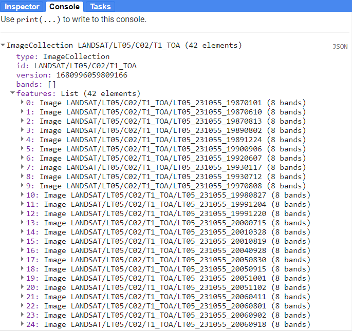
print(lt5)

Checking in the Console, we see that lt5 is an ImageCollection with over 40 images in it.

Let’s do the same thing for Landsat 7, 8, and 9.

// Landsat 7
var le7 = ee.ImageCollection('LANDSAT/LE07/C02/T1_TOA')
    .filterBounds(aoi)
    .filter(ee.Filter.lt('CLOUD_COVER', metadataCloudCoverMax))
    .select(sensorBandDictLandsatTOA['L7'], bandNamesLandsatTOA)

// Landsat 8 
var lc8 = ee.ImageCollection('LANDSAT/LC08/C02/T1_TOA')
    .filterBounds(aoi)
    .filter(ee.Filter.lt('CLOUD_COVER', metadataCloudCoverMax))
    .select(sensorBandDictLandsatTOA['L8'], bandNamesLandsatTOA)

// Landsat 9
var lc9 = ee.ImageCollection('LANDSAT/LC09/C02/T1_TOA')
    .filterBounds(aoi)
    .filter(ee.Filter.lt('CLOUD_COVER', metadataCloudCoverMax))
    .select(sensorBandDictLandsatTOA['L9'], bandNamesLandsatTOA)

Next, we want to apply some functions to each Landsat scene in a collection. In the first function, we will mask clouds and cloud shadows using the QA_PIXEL band that is included in every Landsat scene. The QA_PIXEL band is a bitmask generated in the Landsat processing center before it is distributed to the end-user. It has a lot of useful information contained in it.

We use the cloud and cloud shadow bits for this function.

//--------------------------------------------------------------
// Preprocess images (cloud masking and index calculating)
//--------------------------------------------------------------

// do time series pre-processing using functions that are applied
// every image of the collection

// Create a cloud masking function
function cloudShadowMask(image) {
  // Get the correct bits
  // Bit 3 is cloud, bit 4 is cloud shadow
  var cloudShadowBitMask = (1 << 4);
  var cloudsBitMask = (1 << 3);
  // Get the pixel QA band
  var qa = image.select('QA_PIXEL');
  // Set both flags equal to zero, indicating clear conditions
  var mask = qa.bitwiseAnd(cloudShadowBitMask).eq(0)
             .and(qa.bitwiseAnd(cloudsBitMask).eq(0));
  return ee.Image(image).updateMask(mask);
}

In the second function we generate several spectral indices from the pre-existing spectral bands in our Landsat scenes. All of these indeces can help in identifying mangroves, and index values range from -1 to +1.

NDVI: Normalized Difference Vegetation Index - quantifies vegetation by measuring the difference between near-infrared (which vegetation strongly reflects) and red light (which vegetation absorbs)

LSWI: Land Surface Water Index - calculated as a normalized ratio between near infrared (NIR) and short-wave infrared (SWIR), is sensitive to vegetation and soil water content

NDMI: Normalized Difference Moisture Index - used to determine vegetation water content (calculated as a ratio between the NIR and SWIR values in traditional fashion)

MNDWI: Modified Normalized Difference Water Index - uses green and SWIR bands for the enhancement of open water features (diminishes built-up area features that are often correlated with open water in other indices)

Tip: Here is a great resource published by the University of Bonn for finding indeces for many different purposes: https://www.indexdatabase.de/

// Create function to calculate indices
// NDVI: (NIR-Red)/(NIR+Red)
// LSWI: (NIR-SWIR1)/(NIR+SWIR1)
// NDMI: (SWIR2-Red)/(SWIR2+Red)
// MNDWI: (Green-SWIR2)/(Green+SWIR2)
// We use the GEE function normalizedDifference, expressed as: (b1-b2)/(b1+b2)
function calculateIndices(img){
  var ndvi = img.normalizedDifference(['nir', 'red']).rename('ndvi');
  var lswi = img.normalizedDifference(['nir', 'swir1']).rename('lswi');
  var ndmi = img.normalizedDifference(['swir2', 'red']).rename('ndmi');
  var mndwi = img.normalizedDifference(['green', 'swir2']).rename('mndwi');
  var withIndices = img.addBands(ndvi).addBands(lswi)
                    .addBands(ndmi).addBands(mndwi);
  return withIndices
}

Now let’s apply the functions to every image in each Landsat collection using .map() and see the result.

// Apply pre-processing functions to each image collection
// including cloud masking and index calculating
var lt5_preprocessed = lt5.map(cloudShadowMask)
                              .map(calculateIndices);
var le7_preprocessed = le7.map(cloudShadowMask)
                              .map(calculateIndices);
var lc8_preprocessed = lc8.map(cloudShadowMask)
                              .map(calculateIndices);
var lc9_preprocessed = lc9.map(cloudShadowMask)
                              .map(calculateIndices);                              

//--------------------------------------------------------------
// Visualize a non-processed and pre-processed images
//--------------------------------------------------------------

// Select first non-processed image
var firstNonProcessed = lc8.first();

// Define visualization parameters
var visParamNonProcessed = {
  bands: ['red', 'green', 'blue'],
  min: 0,
  max: 0.2
};

// Add image to map
Map.addLayer(firstNonProcessed, 
            visParamNonProcessed, 
            'First non-processed image');

// Select first pre-processed image
var firstPreProcessed = lc8_preprocessed.first();

// Define visualization parameters
var visParamPreProcessed = {
  bands: ['red', 'green', 'blue'],
  min: 0,
  max: 0.2
};

// Add image to map
Map.addLayer(firstPreProcessed, 
            visParamPreProcessed, 
            'First pre-processed image');

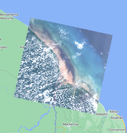
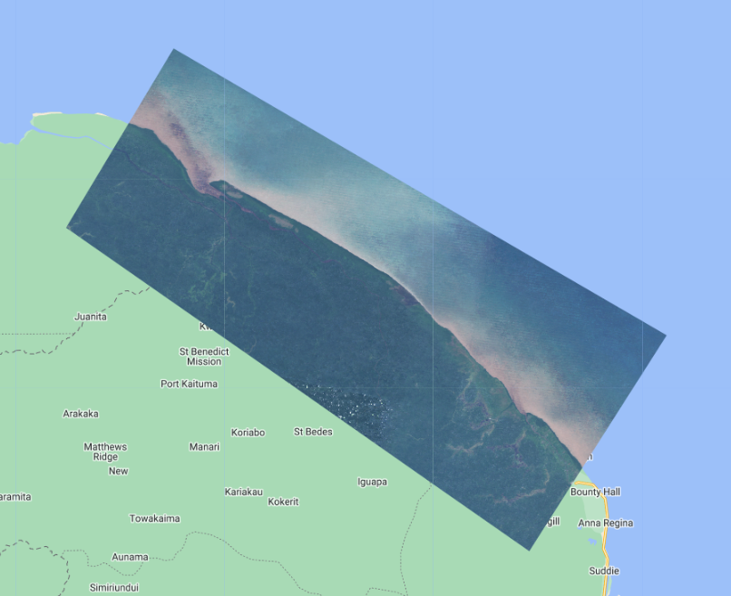
Toggle between the two image layers to see the result of the cloud masking. You can Inspect each image on the map to see that the preprocessed image has a different set of spectral bands than the non-processed image.

Let’s merge our preprocessed Landsat ImageCollections together into one. Finally, we must decide on a specific date range with which we’ll train our Mangrove model. Keep this date range for now, and we’ll experiment later on.

//--------------------------------------------------------------
// Make full Landsat archive in specific date range
//--------------------------------------------------------------

// Merge preprocessed Landsat collections together
var mergedLandsat = lt5_preprocessed
.merge(le7_preprocessed)
.merge(lc8_preprocessed)
.merge(lc9_preprocessed)

// Filter merged collection on date range of interest
// by making a filter object
var dateFilter = ee.Filter.date('2020-01-01','2023-01-01')

// apply filter to merged collections
var landsatFiltered = mergedLandsat.filter(dateFilter)
print(landsatFiltered)

// Add images to the map
Map.addLayer(landsatFiltered,visParamPreProcessed,
             'Landsat Collection 2020-2023', false)

Code Checkpoint: https://code.earthengine.google.com/537c5ab42bbc2088b72de222fb961bb6

We now have an ImageCollection consisting of data from multiple Landsat sensors for your area and date range of interest.

Image Compositing

We’ve now got an ImageCollection consisting of multiple Landsat missions that captured data in our desired date range. To train a mangrove classification model, we’ll reduce the size of our input data by making a composite of the ImageCollection. Let’s make a median composite for this demonstration and clip it to our AOI. Also, let’s add in our DEM and SAR data to this composite.

Note: At a given pixel in your composite, if every single image in your ImageCollection was masked in that location (due to preprocessing in our case), then the composite will also be masked there. This can be remedied by more nuanced preprocessing algorithms and filters for the ImageCollection, but is beyond the scope of this demonstration.

//--------------------------------------------------------------
// Create composite image
//--------------------------------------------------------------

// Use the following functions to compare different aggregations: 
// .min(); .max(); .mean(); .median()
// We will work with the median composite

// Get the median of value of each pixel in the collection
// clipping it to the aoi and adding in the elevation and SAR data
var composite = landsatFiltered
.median()
.clip(aoi)
.addBands(elevation)
.addBands(SARFiltered);

// Add composite to the map
Map.addLayer(composite, visParamPreProcessed, '2020-23 Landsat median composite');

At this point, it is often a good idea to export the input data you have processed for your models. Importing pre-computed data products from a GEE asset will reduce the computational effort required to train and apply models in GEE. It is not necessary for very small AOIs and images with few bands, but this exercise will be too computationally expensive if we don’t do this (GEE will give us an error when we have reached our computational limit). Change the assetId path to one of your own asset folders.

//--------------------------------------------------------------
// Export composite to Drive or Asset
//--------------------------------------------------------------

// // Export composite to Google Drive
// Export.image.toDrive({
//   image: composite.toFloat(),
//   description: 'ToDrivemedianCompositeLandsat_2020-23',
//   fileNamePrefix: 'medianCompositeLandsatDEMSAR_2020-23',
//   region: aoi,
//   scale: 30,
//   maxPixels: 1e13
// });

// Export composite as a GEE Asset
// change assetId to a folder inside your user folder (e.g. users/kwoodward/trinidad-tobago/)
Export.image.toAsset({
  image: composite,
  description: 'ToAssetmedianCompositeLandsat_2020-23',  
  assetId: 'users/ebihari/medianCompositeLandsatDEMSAR_2020-23',
  region: aoi,
  scale: 30,
  maxPixels: 1e13
});

From now on, we will only use the composite imagery we reimport. Make sure to change the path to the correct location of your exported composite.

// Re-import the composite
var composite = ee.Image('users/ebihari/medianCompositeLandsatDEMSAR_2020-23');
// Map.addLayer(composite, visParamPreProcessed, 'Asset');  

Code Checkpoint: https://code.earthengine.google.com/537c5ab42bbc2088b72de222fb961bb6

Continue onto Part 2 to finish your workflow.