Step-Through Part 2
Image Compositing
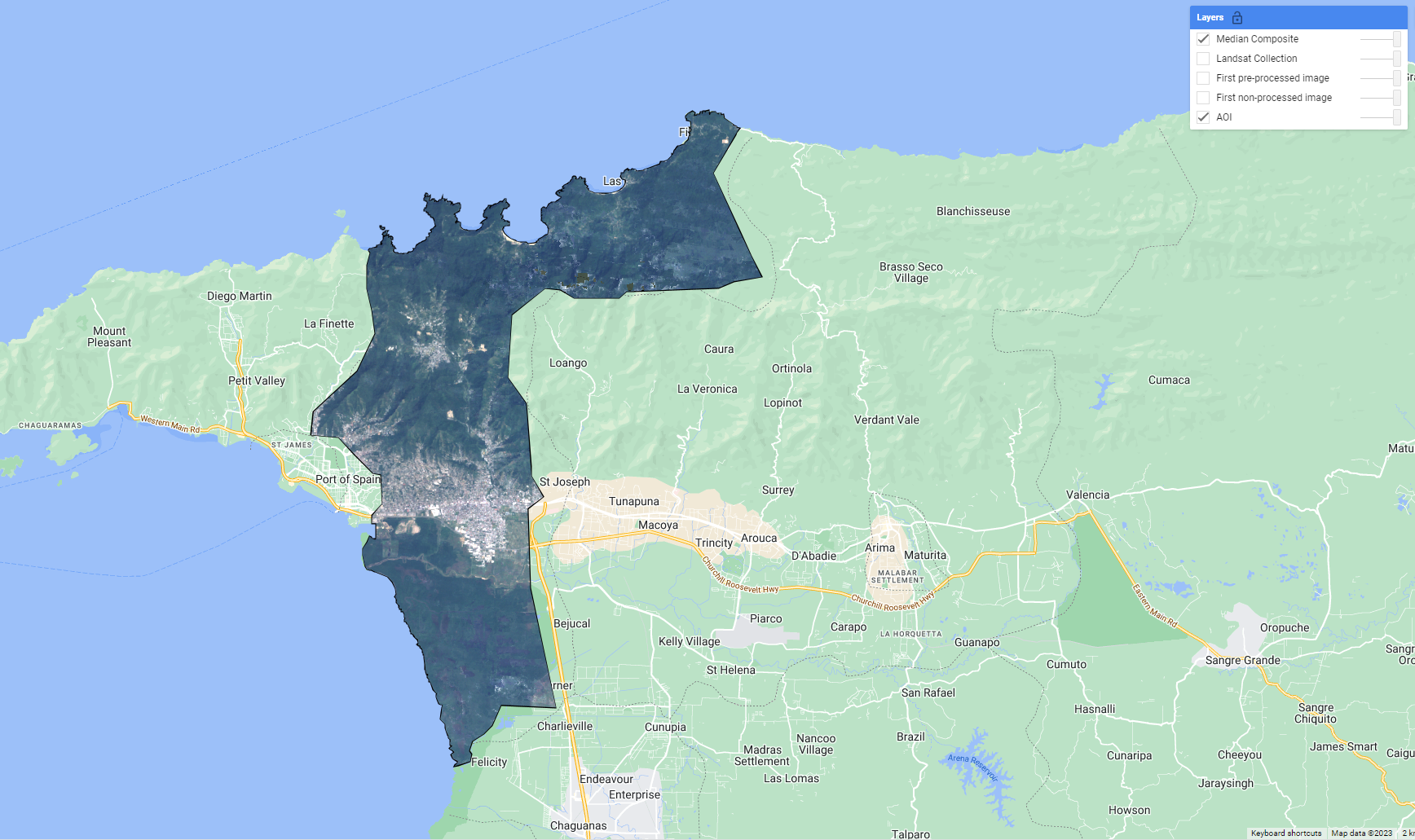
We’ve now got an ImageCollection consisting of multiple Landsat missions that captured data in our desired date range. To train a mangrove classification model, we’ll reduce the size of our input data by making a composite of the ImageCollection. Let’s make a median composite for this demonstration and clip it to our AOI.
Note: At a given pixel in your composite, if every single image in your ImageCollection was masked in that location (due to preprocessing in our case), then the composite will also be masked there. This can be remedied by more nuanced preprocessing algorithms and filters for the ImageCollection, but is beyond the scope of this demonstration.
//--------------------------------------------------------------
// Create a composite image
//--------------------------------------------------------------
// Use the following functions to compare different aggregations:
// .min(); .max(); .mean(); .median()

// We will work with the Median composite.
var composite = landsatFiltered.median().clip(aoi);

// Add composite to the map.
Map.addLayer(composite, visParamPreProcessed, 'Median Composite');
At this point, sometimes it is a good idea to export the input data you have processed for your models. Importing pre-computed data products from a GEE asset will reduce the computational effort required to train and apply models in GEE. It is not necessary for this demonstration with such a small AOI, but bear that in mind for future work. If you decide to export your composite to a GEE asset, please change the assetId path to one of your own asset folders.
//--------------------------------------------------------------
// Export composite to Drive or Asset
//--------------------------------------------------------------

// Export composite to Google Drive.
Export.image.toDrive({
  image: composite.toFloat(),
  description: 'ToDrivemedianCompositeLandsat_2000_05_Caroni',
  fileNamePrefix: 'medianCompositeLandsat_2000_05_Caroni',
  region: aoi,
  scale: 30,
  maxPixels: 1e13
});

// Export composite as a GEE Asset.
// change assetId to a folder inside your user folder (e.g. users/kwoodward/trinidad-tobago/)
Export.image.toAsset({
  image: composite,
  description: 'ToAssetmedianCompositeLandsat_2000_05_Caroni',
  assetId: 'projects/caribbean-trainings/assets/trinidad-tobago-2022/images/medianCompositeLandsat_2000_05_Caroni',
  region: aoi,
  scale: 30,
  maxPixels: 1e13
});

// Re-import median composite.
// var asset = ee.Image('projects/caribbean-trainings/assets/trinidad-tobago-2022/images/medianCompositeLandsat_2000_05_Caroni');
// Map.addLayer(asset, visParamPreProcessed, 'Asset');
Sample Data
To train a mangrove classification model, we need presence/absence data on the locations of mangroves. There are several widely cited mangrove datasets out there now. The Giri et al 2011 dataset is already in the GEE data catalog, it contains a mangrove extent map circa 2000.
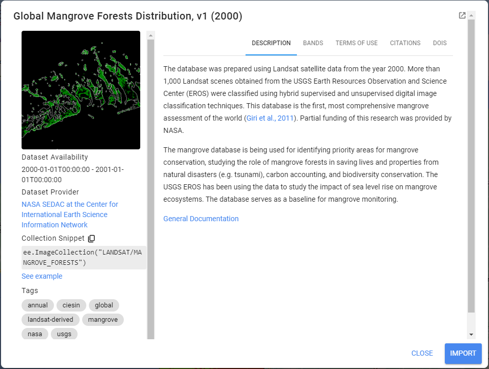
This dataset is an ImageCollection containing tiled raster data. Let’s mosaic the tiles together, clip it to our AOI and check it out.
//--------------------------------------------------------------
// Training data
//--------------------------------------------------------------

// We will auto-generate Mangrove presence-absence reference points from the Giri et al 2000 Mangrove Extent Map
// Process the Mangrove Forests imageCollection into a clipped raster
var giriMangrovesTT = ee.ImageCollection("LANDSAT/MANGROVE_FORESTS")
.filterBounds(aoi)
.mosaic()
.unmask(0)
.clip(aoi)
.rename('class')

Map.addLayer(giriMangrovesTT,{min:0,max:1},'Giri Mangrove Extent Map T&T',false)
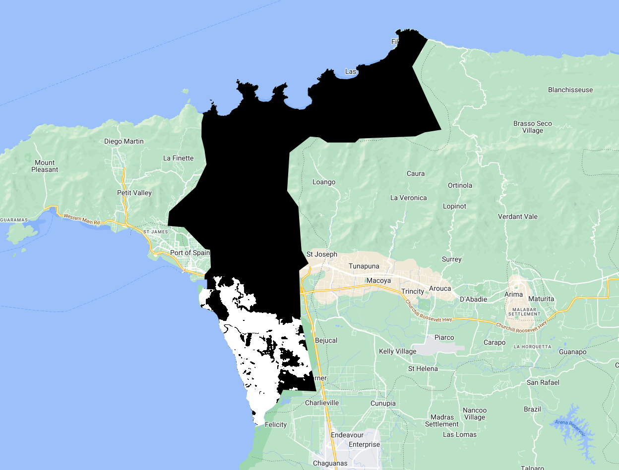
Now that we have a presence/absence mangrove map, we can draw reference samples which will be used to train and validate our mangrove classification. First, lets generate a stratified sample of presence and absence points from the magrove presence/absence raster. We specify that we want 100 points of Mangrove and 100 points of Not Mangrove.
// sample from the processed mangrove raster. Values in 'class' property:  0-Not Mangrove,  1-Mangrove
var collectedPts = giriMangrovesTT.stratifiedSample({
  numPoints:100,
  classBand:'class',
  region:aoi,
  scale:30,
  projection:'EPSG:3857',
  seed:01010,
  classValues:[0,1],
  classPoints:[100,100],
  dropNulls:true,
  tileScale:2,
  geometries:true});
print('Collected Points', collectedPts)
// Optionally you can export and re-import it
// Export.table.toAsset(referencePts,'mangroveSamples','projects/caribbean-trainings/assets/trinidad-tobago-2022/referencePoints_GiriMangroves_100ea')
// var collectedPts = ee.FeatureCollection("projects/caribbean-trainings/assets/trinidad-tobago-2022/referencePoints_GiriMangroves_100ea")
Next, we must extract the raster values of the Landsat composite to each reference point. Let’s see what we have in trainingPts.
// Extract spectral information at each point.
var trainingPts = composite.sampleRegions({
    collection: collectedPts,
    properties: ['class'],
    scale: 30,
    geometries:true
  });
print('Training Points', trainingPts);
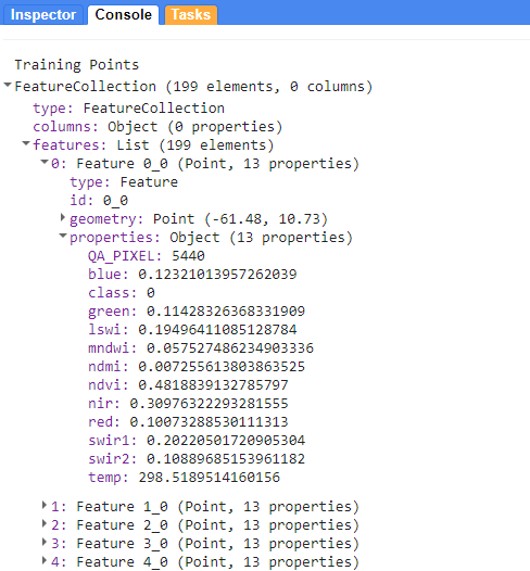
Each point within the FeatureCollection contains the value of the underlying pixel for every band in our Landsat composite image. Each band’s name and value is stored as a property in the point feature.
Classification
Now that we have generated our image composite and our training data, it is time to train the Random Forest and classify our composite with it.
// Define prediction bands.
var predictionBands =  landsatFiltered.first().bandNames().remove('QA_PIXEL'); // all image bands except the QA band
print('Prediction Bands',predictionBands)

// Random Forest Classifier.
// "Call" the random forest classifier and train it with the training points.
var RFclassifier = ee.Classifier.smileRandomForest({numberOfTrees:10}).train({
  features: trainingPts,
  classProperty: 'class',
  inputProperties: predictionBands
});

// Print decision trees.
var decisionTrees = RFclassifier.explain();
print('Decision trees', decisionTrees);

// Define color palette for the classified image (grab from geometry tools for each class).
var colorPalette = ['d63000', '98ff00'];

// Classify the median composite.
var RFclassification = composite
.select(predictionBands)
.classify(RFclassifier);

Map.addLayer(RFclassification, {min: 0, max: 1, palette: colorPalette}, 'RF Classification');
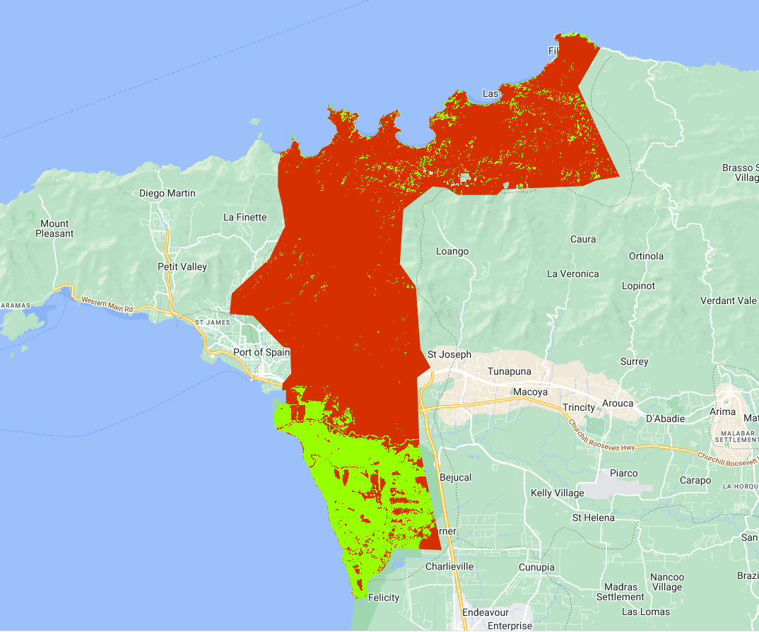
How does it look? Let’s quantify how well the classification did with an initial accuracy assessment. We will do this with the trainingPts FeatureCollection. We first split it out into 80% training points, 20% testing points.
//--------------------------------------------------------------
// Pre-validation
//--------------------------------------------------------------
// Divide points into training and testing points.
// Create random column in reference points.
var trainingTesting = trainingPts.randomColumn();
print(trainingTesting);
// Divide 80% of data for training and 20% for testing.
var trainingData = trainingTesting.filter(ee.Filter.lt('random', 0.8));
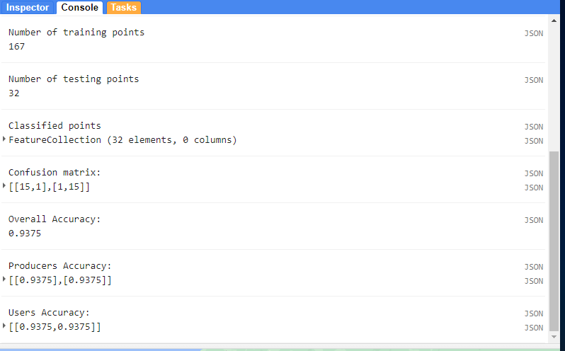
print('Number of training points', trainingData.size());
var testingData = trainingTesting.filter(ee.Filter.gte('random', 0.8));
print('Number of testing points', testingData.size());
Map.addLayer(trainingData, {color: '429ef5'}, 'Training points'); // Blue
Map.addLayer(testingData, {color: '000000'}, 'Testing points'); // Black
We train a Random Forest classifier with only the training point subset this time. Then we take this trained RF classifer to classify the testing point subset. Finally, we retrieve the error matrix from the classified test set and print accuracy metrics to the console.
// Train the classifier with training points only.
var RFclassifierVal = ee.Classifier.smileRandomForest(10).train({
  features: trainingData,
  classProperty: 'class',
  inputProperties: predictionBands
});

// Now, test the classification (model precision) with testing data.
var classificationVal = testingData.classify(RFclassifierVal);
print('Classified points', classificationVal);

// Create confusion matrix.
var confusionMatrix = classificationVal.errorMatrix({
  actual: 'class',
  predicted: 'classification'
});

// Print Confusion Matrix and accuracies.
print('Confusion matrix:', confusionMatrix);
print('Overall Accuracy:', confusionMatrix.accuracy());
print('Producers Accuracy:', confusionMatrix.producersAccuracy());
print('Users Accuracy:', confusionMatrix.consumersAccuracy());
Code Checkpoint: https://code.earthengine.google.com/332194d54f2ccdfec00257cc08abc8b1
Congratulations! You have setup a Random Forest classifier for mangrove mapping using multiple Landsat sensors.