Step-Through Part 1
Overview
In this workflow, we will create an archive of Landsat imagery from Landsat missions 5 through 9, filter the image archive down to a desired time period of interest, then use the data to classify mangrove presence using a Random Forest classification model.
Follow along by copying and pasting each code block in the lesson into your own blank script. At the end you will have the entire workflow saved to a script file on your own GEE account.
Setting up Area of Interest
An area of interest can be uploaded from a local shapefile, drawn on the map, or derived from a pre-existing dataset in the Earth Engine catalogue. Here we will use the Food and Agriculture Organization’s Global Administrative Units Layer (FAO GAUL) dataset to derive our AOI. At the top of the code editor, type in the search bar ‘FAO GAUL Global First’. We see that it is a FeatureCollection containing Level 1 administrative boundaries globally.
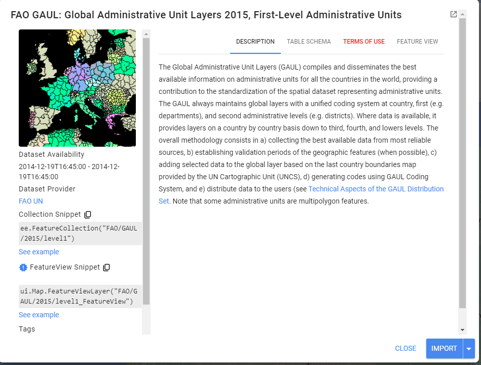
Click on the Table Schema tab. We notice there is a useful field named ‘ADM1_NAME’. We will use this property to derive our AOI. We will focus in on the San Juan area and the mangrove area to its south.
//--------------------------------------------------------------
// Define vector data (Area of interest, aoi)
//--------------------------------------------------------------
// Define variable region by filtering the FAO dataset.
// https://developers.google.com/earth-engine/datasets/catalog/FAO_GAUL_2015_level1
var boundaries = ee.FeatureCollection("FAO/GAUL/2015/level1");
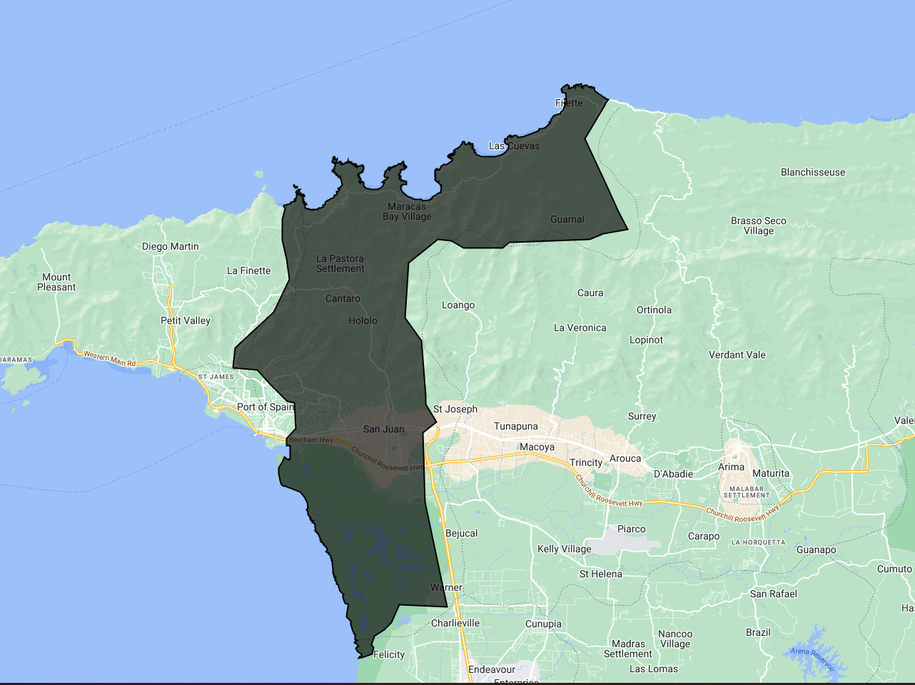
var aoi = boundaries.filter(ee.Filter.eq('ADM1_NAME', 'San Juan/Laventille'));
// Center the Map on the aoi object, with a specified zoom-level (between 1-24)
Map.centerObject(aoi, 12);
// Add the aoi object as a layer to the map
Map.addLayer(aoi, {}, 'AOI');
Preprocessing Image Collections
We always want to apply filters to ImageCollections as early in our workflow as we can to reduce the amount of effort the GEE servers will require. We already know the area that we’d like to pull data for (our AOI), and that we want relatively few clouds in our images, so we will apply a boundary and a cloud cover filter.
Let’s do that for our first Landat ImageCollection
//--------------------------------------------------------------
// Define raster data
//--------------------------------------------------------------
// We will merge together all Landsat Image Collections from Landsat 4 to Landsat 9
// to make a continuous archive of data going back to the 1990s
// Each Landsat imageCollection has slightly different ordering of bands
// handling it with a dictionary saves us some typing
var sensorBandDictLandsatTOA = {'L9': [1, 2, 3, 4, 5, 9, 6, 11],
'L8': [1, 2, 3, 4, 5, 9, 6, 11],
'L7': [0, 1, 2, 3, 4, 5, 7, 9],
'L5': [0, 1, 2, 3, 4, 5, 6, 7],
'L4': [0, 1, 2, 3, 4, 5, 6, 7]}
var bandNamesLandsatTOA = ['blue', 'green',
'red', 'nir', 'swir1', 'temp', 'swir2', 'QA_PIXEL']
// filter by max cloud cover % in a scene
var metadataCloudCoverMax = 25
// Landsat 5
var lt5 = ee.ImageCollection('LANDSAT/LT05/C02/T1_TOA')
.filterBounds(aoi)
.filter(ee.Filter.lt('CLOUD_COVER', metadataCloudCoverMax))
.select(sensorBandDictLandsatTOA['L5'], bandNamesLandsatTOA)
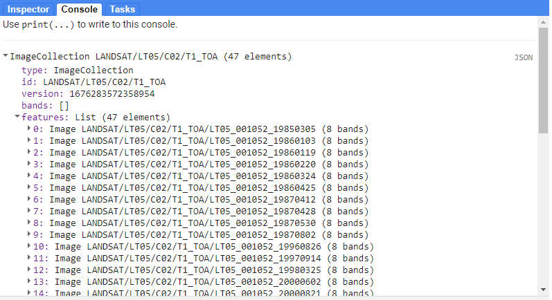
print(lt5)
Checking in the Console, we see that lt5 is an ImageCollection with over 40 images in it.
Tip: Since there are differences in the amount and the order of bands on each Landsat mission, we use a dictionary (sensorBandDictLandsatTOA) and a list (bandNamesLandsatTOA) to standardize this information for us going forward using select() - it saves us quite a bit of typing when doing this for multiple collections.
Let’s do the same thing for Landsat 7, 8, and 9.
// Landsat 7
var le7 = ee.ImageCollection('LANDSAT/LE07/C02/T1_TOA')
    .filterBounds(aoi)
    .filter(ee.Filter.lt('CLOUD_COVER', metadataCloudCoverMax))
    .select(sensorBandDictLandsatTOA['L7'], bandNamesLandsatTOA)

// Landsat 8
var lc8 = ee.ImageCollection('LANDSAT/LC08/C02/T1_TOA')
    .filterBounds(aoi)
    .filter(ee.Filter.lt('CLOUD_COVER', metadataCloudCoverMax))
    .select(sensorBandDictLandsatTOA['L8'], bandNamesLandsatTOA)

// Landsat 9
var lc9 = ee.ImageCollection('LANDSAT/LC09/C02/T1_TOA')
    .filterBounds(aoi)
    .filter(ee.Filter.lt('CLOUD_COVER', metadataCloudCoverMax))
    .select(sensorBandDictLandsatTOA['L9'], bandNamesLandsatTOA)
Next, we want to apply some functions to each Landsat scene in a collection. In the first function, we will mask clouds and cloud shadows using the QA_PIXEL band that is included in every Landsat scene. The QA_PIXEL band is a bitmask generated in the Landsat processing center before it is distributed to the end-user. It has a lot of useful information contained in it.
![]()
We use the cloud and cloud shadow bits for this function.
//----------------------------------------------------------
// Time series pre-processing using functions that are applied
// to each and every image of the collection.
//----------------------------------------------------------

// Cloud masking function.
function cloudShadowMask(image) {
  // Bits 3 and 4 are cloud and cloud shadow, respectively.
  var cloudShadowBitMask = (1 << 4);
  var cloudsBitMask = (1 << 3);
  // Get the pixel QA band.
  var qa = image.select('QA_PIXEL');
  // Both flags should be set to zero, indicating clear conditions.
  var mask = qa.bitwiseAnd(cloudShadowBitMask).eq(0)
                .and(qa.bitwiseAnd(cloudsBitMask).eq(0));

  return ee.Image(image).updateMask(mask);
}
In the second function we generate several spectral indices from the pre-existing spectral bands in our Landsat scenes.
// Function to calculate indices
// NDVI: (NIR-Red)/(NIR+Red)
// LSWI: (NIR-SWIR1)/(NIR+SWIR1)
// NDMI: (SWIR2-Red)/(SWIR2+Red)
// MNDWI: (Green-SWIR2)/(Green+SWIR2)
// We use the GEE function normalizedDifference, expressed as: (b1-b2)/(b1+b2)
function calculateIndices(img){
  var ndvi = img.normalizedDifference(['nir', 'red']).rename('ndvi');
  var lswi = img.normalizedDifference(['nir', 'swir1']).rename('lswi');
  var ndmi = img.normalizedDifference(['swir2', 'red']).rename('ndmi');
  var mndwi = img.normalizedDifference(['green', 'swir2']).rename('mndwi');
  var withIndices = img.addBands(ndvi).addBands(lswi).addBands(ndmi).addBands(mndwi);
  return withIndices
}
Now let’s apply the functions to every image in each Landsat collection using .map() and see the result.
// Apply pre-processing functions to each image collection.

var lt5_preprocessed = lt5.map(cloudShadowMask)
                              .map(calculateIndices);
var le7_preprocessed = le7.map(cloudShadowMask)
                              .map(calculateIndices);
var lc8_preprocessed = lc8.map(cloudShadowMask)
                              .map(calculateIndices);
var lc9_preprocessed = lc9.map(cloudShadowMask)
                              .map(calculateIndices);

//--------------------------------------------------------------
// Visualize a non-processed and pre-processed image
//--------------------------------------------------------------

// Select first non-processed image.
var firstNonProcessed = lc8.first();

// Define visualization parameters.
var visParamNonProcessed = {
  bands: ['red', 'green', 'blue'],
  min: 0,
  max: 0.2
};

// Add image to map.
Map.addLayer(firstNonProcessed,
            visParamNonProcessed,
            'First non-processed image');


// Select first pre-processed image.
var firstPreProcessed = lc8_preprocessed.first();

// Define visualization parameters.
var visParamPreProcessed = {
  bands: ['red', 'green', 'blue'],
  min: 0,
  max: 0.2
};

// Add image to map.
Map.addLayer(firstPreProcessed,
            visParamPreProcessed,
            'First pre-processed image');
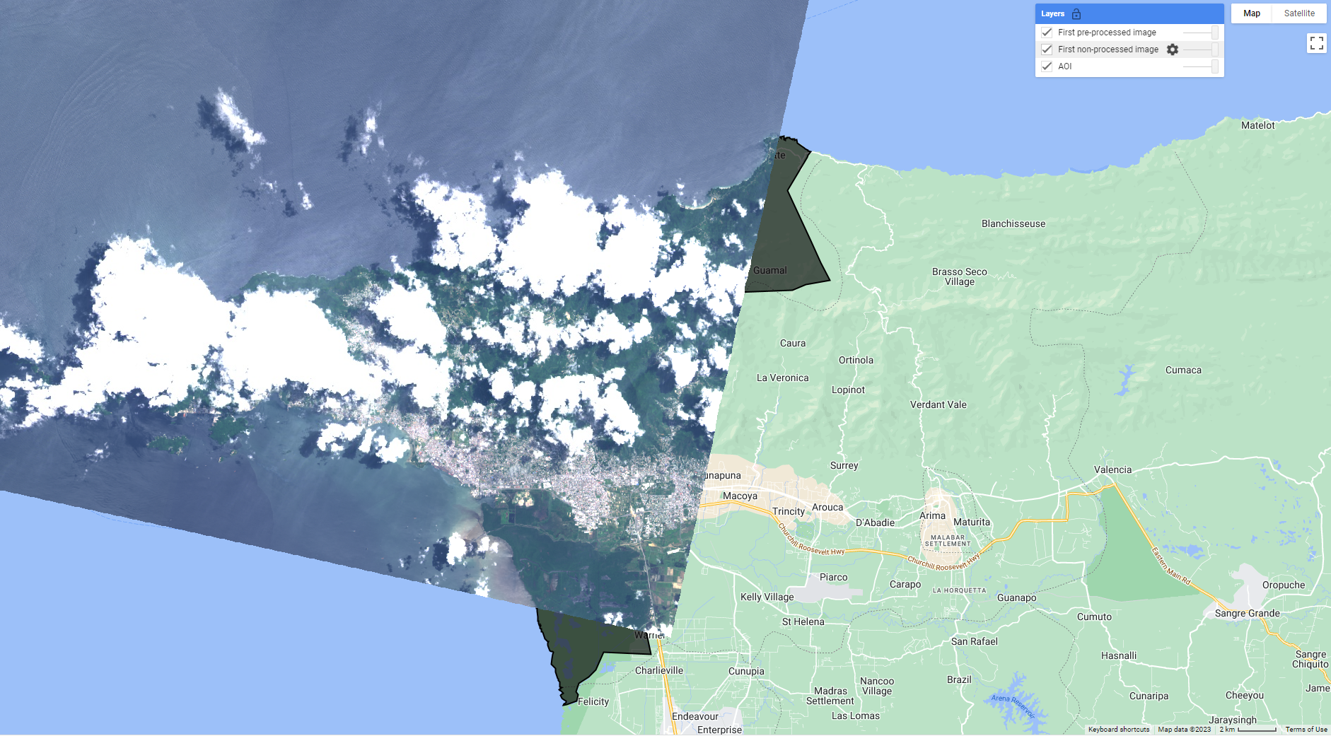
Toggle between the two image layers to see the result of the cloud masking. You can Inspect each image on the map to see that the preprocessed image has a different set of spectral bands than the non-processed image.
Let’s merge our preprocessed Landsat ImageCollections together into one. Finally, we must decide on a specific date range with which we’ll train our Mangrove model. Keep this date range for now, and we’ll experiment later on.
//--------------------------------------------------------
// Make Full Landsat Archive in your Date Range of Interest
//---------------------------------------------------------

// Merge preprocessed Landsat collections together
var mergedLandsat = lt5_preprocessed
.merge(le7_preprocessed)
.merge(lc8_preprocessed)
.merge(lc9_preprocessed)

// Filter merged collection on date range of interest
// make a filter object
var dateFilter = ee.Filter.date('2000-01-01','2005-01-01')

// apply filter
var landsatFiltered = mergedLandsat.filter(dateFilter)
print(landsatFiltered)
Map.addLayer(landsatFiltered,{},'Landsat Collection',false)
Code Checkpoint: https://code.earthengine.google.com/0064c2b2764e781d4f8f1abf9c59f762
Congratulations, you now have an ImageCollection consiting of data from multiple Landsat sensors for your area and date range of interest. Continue onto Step Through Part 2 to finish your workflow.