Script
The script of this section is available here.
Dataset Identification and Preparation
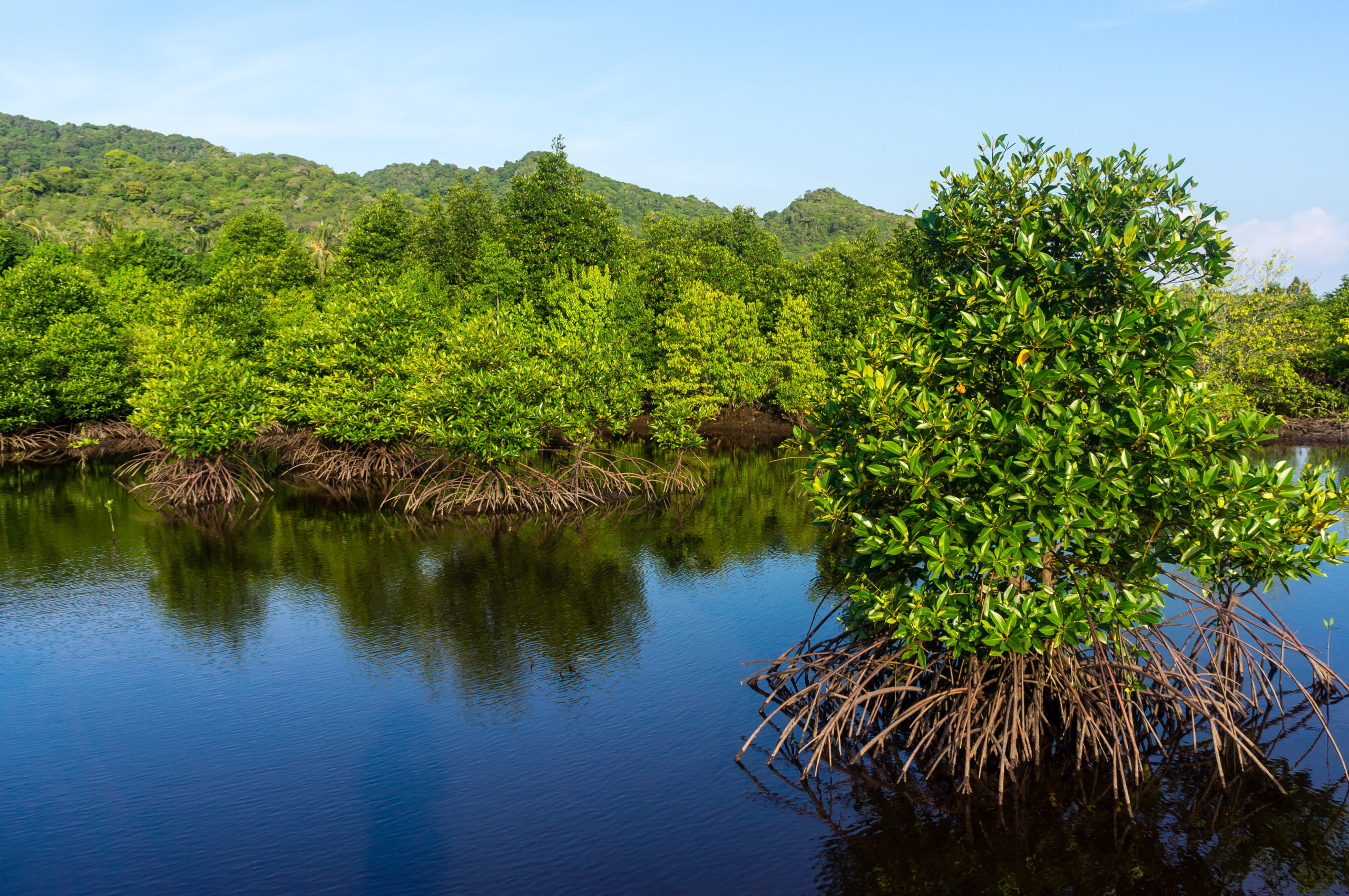
Before running any habitat mapping it is important to identify the type of data and processing we require to achieve the best possible outcome. In this case we will use data available in the catalog of GEE for mapping mangroves in Suriname. The mangrove trees grow in coastal areas, this means we can focus on those areas and there is no need to search for mangroves in inland or highland areas.
We first have to identify the data that best satisty our needs, for example: what pixel, temporal or spectral resolution is better? We will use multispectral data from Sentinel-2, which delivers data at 10 m per pixel every ~5 days from ~2016 to present.
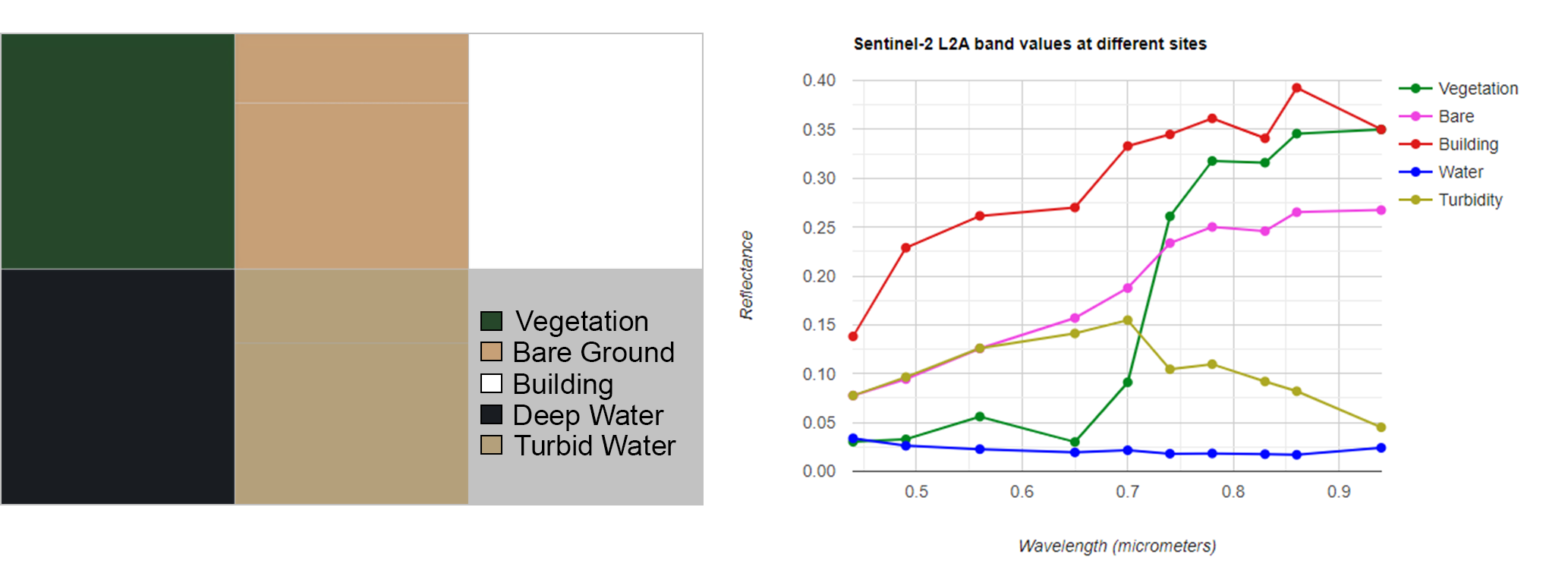
The mangrove trees have a spectral signature, which can help us to disguinsh and separate them from other objects. However, those spectral signatures in multispectral data may be limited by the number of bands available, which can make difficult to separate some objects or classes from others.
Additionally, the mangrove mapping may use other ancillary data to increase mapping performance. In this we will use digital elevation data (DEM), normalized difference vegetation index (NDVI), and normalized difference water index (NDWI). Previously known mangrove distribution is useful to delimitate our mapping area nad to collect sampling points. The global mangrove distribution is available in GEE and it was produced by using Landsat imagery at 30 m per pixel.
Steps
The steps for this section are:
- Identify datasets of interest:
- Multispectral collection
- DEM data
- Mangrove global distribution dataset
- NDVI (Calculate in step 3)
- NDWI (Calculate in step 3)
- Create cloudless composite image
- Calculate NDVI & NDWI from composite
- Export images of interest
1. Load datasets of interest
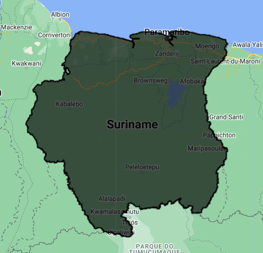
We will load the LSIB 2017 collection of international boundary polygons and select the polygon that corresponds to Suriname. The property containing country names is COUNTRY_NA.
// Define country boundaries
var suriname = ee.FeatureCollection("USDOS/LSIB/2017")
                .filter(ee.Filter.eq('COUNTRY_NA','Suriname'));
// Visualize feature
Map.addLayer(suriname, {}, 'Suriname');
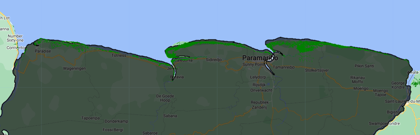
Now, let’s load the Global mangrove distribution dataset, which is derived from Landsat imagery from 2000 at 30 m per pixel. We will focus on Suriname.
/////////  Global Mangrove Distribution Data  //////////
var globalMangrove = ee.ImageCollection("LANDSAT/MANGROVE_FORESTS");

// Visualize mangrove dataset:
Map.addLayer(globalMangrove, {palette:['green']}, 'Global Mangrove');
The next collection is the Global DEM from Copernicus at 30 m per pixel. This collection contain several bands and we have to make sure to select the DEM band. We will clip the DEM to show only valid data in Suriname and will explore the best way to visualize this data (e.g. identify minimum and maximum elevations).
/////////  Digital Elevation Model at 30m  //////////
var dem = ee.ImageCollection("COPERNICUS/DEM/GLO30").select('DEM');

// Clip and Visualize DEM:
var demSuriname = dem.mosaic().clip(suriname);
var demPalette = ['#002bff','#00f3ff','#00ff37','#fbff00','#ff0000'];
Map.addLayer(demSuriname, {palette: demPalette, min:0, max:850}, 'DEM');

Finally, we will load the Sentinel-2 L2A multispectral data at 10 m per pixel. This collection require some preprocessing before using for mangrove mapping. We will define the time range of interest, study area, and cloud percentage per image. If we set the location to Suriname, time range to filterDate('2019-01-01','2023-12-31'), and cloud percentage to less than 20%, we will obtain a collection of 807 images.
////////////  Multispectral data: Sentinel-2 at 10m  /////////////
var sentinel2 = ee.ImageCollection("COPERNICUS/S2_SR_HARMONIZED");

var s2Suriname = sentinel2.filterBounds(suriname)
                          .filterDate('2019-01-01','2023-12-31')
                          .filter(ee.Filter.lt('CLOUDY_PIXEL_PERCENTAGE',20));

print('Sentinel-2 collection', s2Suriname);
2. Cloudless Composite
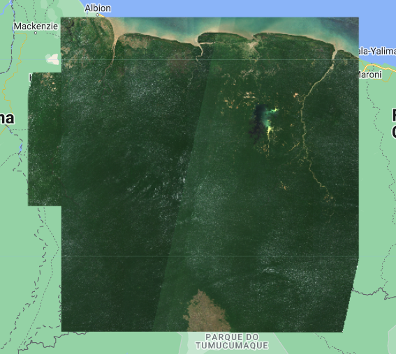
After filtering the Sentinel-2 collection we can apply a cloud mask function to clean any clouds, and finally we can create a composite. The composite will be clipped to a define area of interest defined in the variable aoi. Note that clouds are sometimes hard to remove from certain areas.
// Function for masking clouds of Sentinel-2 images
function maskS2clouds(image) {
  var qa = image.select('QA60'); // Select QA bands

  // Bits 10 y 11 are clouds and cirrus, respectively.
  // The sign << is the "bitwise shift" operator
  var cloudBitMask = 1 << 10;  // 1+10 zeros, equal to 1024, opaque clouds
  var cirrusBitMask = 1 << 11; // 1+11 zeros, equal to 2048, cirrus

  // Transform bits, get zero values and create mask, which means cloudless pixels.
  var mask = qa.bitwiseAnd(cloudBitMask).eq(0)
             .and(qa.bitwiseAnd(cirrusBitMask).eq(0));

  // Apply mask
  return image.updateMask(mask);
}

// Define an area of interest
var aoi =
    /* color: #d63000 */
    /* shown: false */
    /* displayProperties: [
      {
        "type": "rectangle"
      }
    ] */
    ee.Geometry.Polygon(
        [[[-58.37382276058198, 6.217798510145414],
          [-58.37382276058198, 1.6155669446230103],
          [-53.64970166683198, 1.6155669446230103],
          [-53.64970166683198, 6.217798510145414]]], null, false);
Map.addLayer(aoi, {}, 'AOI');

// Apply cloud mask function, get median values, and clip to the Suriname boundary.
var s2Cloudless = s2Suriname.map(maskS2clouds)
                            .median()
                            .clip(aoi);

// Visualize map
var visParams = {bands: ['B4','B3','B2'], min:0, max:2000};
Map.addLayer(s2Cloudless, visParams, 'Composite');
3. Calculate NDVI & NDWI from composite
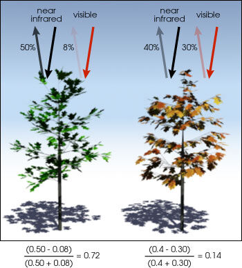
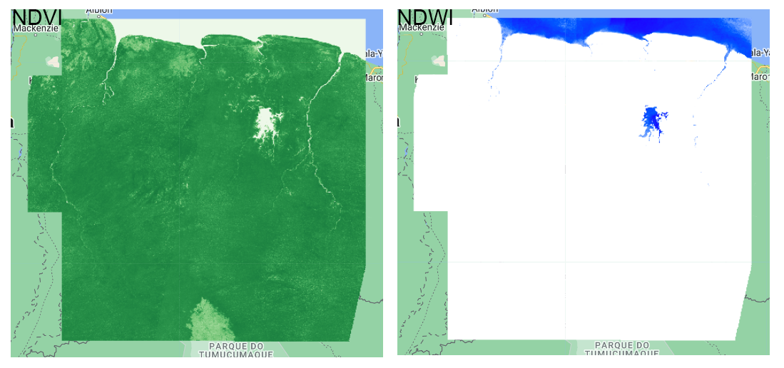
NDVI: Normalized Difference Vegetation Index
The NDVI values range from -1 to +1. Tipically, negative NDVI values may indicate presence of water bodies. In the other side, if the NDVI values are closer to +1 it is very likey this is indicating dense vegetation. When the NDVI is closer to zero it may indicate urban areas.
We use the following equation to obtain NDVI:
\[\frac{(NIR-RED)}{(NIR+RED)}\]The ratio between the NIR and RED bands provide a vegetation index:
NDWI: Normalized Difference Water Index
This index allows to detect water bodies using the GREEN and NIR bands. The water allows deeper penetration of shorter wavelenghts such as blue and green, in comparison to longer wavelenghts such as red or infrared. However, this optical properties may be altered by content of other elements in water such as colored dissolved organic matter, suspended particles, or algal concentration. The threshold for water detection is around 0.3, where equal or higher values indicate the presence of water.
The equation to obtain NDWI is:
\[\frac{(GREEN-NIR)}{(GREEN+NIR)}\]// Calculate NDVI and NDWI
var ndvi = s2Cloudless.normalizedDifference(['B8','B4']).rename('NDVI');
var ndwi = s2Cloudless.normalizedDifference(['B3','B8']).rename('NDWI');
// Visualize layers
var ndviPalette = ['#edf8e9','#c7e9c0','#a1d99b','#74c476','#41ab5d','#238b45','#005a32'];
var ndwiPalette = ['#ffffff','#0059ff','#1d00ff','#0c00b0'];
Map.addLayer(ndvi, {palette:ndviPalette,min:0,max:1}, 'NDVI');
Map.addLayer(ndwi, {palette:ndwiPalette,min:0,max:1}, 'NDWI');
4. Export images
We will export the Sentinel-2 composite, NDVI and NDWI images to our personal assets. The argument assetId is where we specfify the folder and file name to save. Other arguments are important such as the scale, crs, region, maximum of pixels. Once we run the script we need to go to teh Tasks tab, hit run and submit the task to the GEE server. We can monitor the submitted tasks whenever we want in this section.
//// Export Images to Assets:

// Sentinel-2 Map
Export.image.toAsset({
  image: s2Cloudless,
  description: 'Sentinel2_Suriname_Map',
  assetId: 'Suriname/Suriname_Map',
  region: aoi,
  scale: 10,
  crs: 'EPSG:4326',
  maxPixels: 1e13
});

// NDVI Map
Export.image.toAsset({
  image: ndvi,
  description: 'NDVI_Suriname_Map',
  assetId: 'Suriname/NDVI_Map',
  region: aoi,
  scale: 10,
  crs: 'EPSG:4326',
  maxPixels: 1e13
});

// NDWI Map
Export.image.toAsset({
  image: ndwi,
  description: 'NDWI_Suriname_Map',
  assetId: 'Suriname/NDWI_Map',
  region: aoi,
  scale: 10,
  crs: 'EPSG:4326',
  maxPixels: 1e13
});

After exporting this data we will be all set to start with the next section of collecting training data.