Run Classification and Calculate Change
Visualize Spectral Signatures
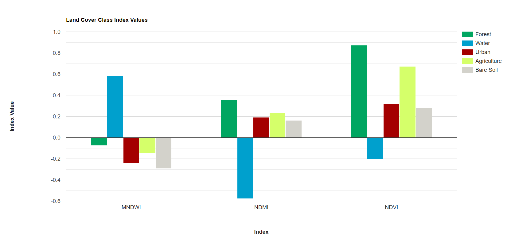
Before beginning our analysis, we quickly visualize the spectral signatures and index values of our representative polygons of different land cover classes. We use Earth Engine’s ui.Chart functionality to graph the median values of the bands and indices for each land cover class. Do the spectral signatures look different between our 5 classes? Are there any classes that are very similar to each other, and thus might be difficult to separate in our random forest model?
//--------------------------------------------------------------
// Visualize spectral signatures
//--------------------------------------------------------------

// Convert sample polygon featureCollection to an image
var year1_FC_image =
    year1_FC
        .reduceToImage({properties: ['landcover'], reducer: ee.Reducer.first()})
        .rename('landcover');

// Select the Landsat bands you want to display
var preImage_forchart = preImage.select(['blue', 'green', 'red', 'nir', 'swir1', 'swir2'])
    // Add the sample polygons image bands on to the Landsat composite
    .addBands(year1_FC_image);

// Define the list of bands to be the x-axis labels
//(based on wavelength in micrometers)
var bands = ['blue', 'green', 'red', 'NIR', 'SWIR1', 'SWIR2'];
var wavelenghts = [0.47, 0.56, 0.65, 0.86, 1.6, 2.2]

// Define the chart and print it to the console
var chart = ui.Chart.image
                .byClass({
                  image: preImage_forchart,
                  classBand: 'landcover',
                  region: year1_FC,
                  reducer: ee.Reducer.median(),
                  scale: 30,
                  classLabels: ['','Forest', 'Water', 'Urban', 'Agriculture', 'Bare Soil'],
                  xLabels: wavelenghts
                })
                //.setChartType('ScatterChart')
                .setChartType('ScatterChart')
                .setOptions({
                  title: 'Land Cover Class Spectral Signatures',
                  hAxis: {
                    title: 'Band Wavelength (µm)',
                    titleTextStyle: {italic: false, bold: true},
                    ticks: wavelenghts
                  },
                  vAxis: {
                    title: 'Reflectance',
                    titleTextStyle: {italic: false, bold: true}
                  },
                  colors: ['00a661','00a0cd','a40000', 'd5ff6a','d3d2cb'],
                  pointSize: 0,
                  lineSize: 2,
                  curveType: 'linear'
                });
print(chart);

// Select the Landsat indices you want to display
var preImage_forchart2 = preImage.select(['ndvi', 'mndwi', 'ndmi'])
    // Add the sample polygons image bands on to the Landsat composite
    .addBands(year1_FC_image);

// Define the list of bands to be the x-axis labels
var bands2 = ['NDVI', 'MNDWI', 'NDMI'];

// Define the chart and print it to the console
var chart2 = ui.Chart.image
                .byClass({
                  image: preImage_forchart2,
                  classBand: 'landcover',
                  region: year1_FC,
                  reducer: ee.Reducer.mean(),
                  scale: 30,
                  classLabels: ['','Forest', 'Water', 'Urban', 'Agriculture', 'Bare Soil'],
                  xLabels: bands2
                })
                .setChartType('ColumnChart')
                .setOptions({
                  title: 'Land Cover Class Index Values',
                  hAxis: {
                    title: 'Index',
                    titleTextStyle: {italic: false, bold: true}
                  },
                  vAxis: {
                    title: 'Index Value',
                    titleTextStyle: {italic: false, bold: true}
                  },
                  colors: ['00a661','00a0cd','a40000', 'd5ff6a','d3d2cb']
                });
print(chart2);

Run Random Forest Classification
We choose a classifier algorithm from ee.Classifier family of functions, and train it on the training_y1 and training_y2 FeatureCollections with train(). We must specify the classProperty to be the property we want to map, or predict, with the model, and the inputProperties as the Landsat band and index values defined by the predictionBands variable. Then, we run the classifier on the preImage and postImage with classify().
We use a Random Forest classifier, which puts each individual pixel through many decision trees (with some random element to them) that each place the pixel in one of our pre-defined classes based on the pixel’s spectral similarity to our training points. The final class of the pixel will be the class that the majority of the decision trees gave that pixel. We print out our decision trees to see how the classifier decided to categorize pixels based on their spectral values.
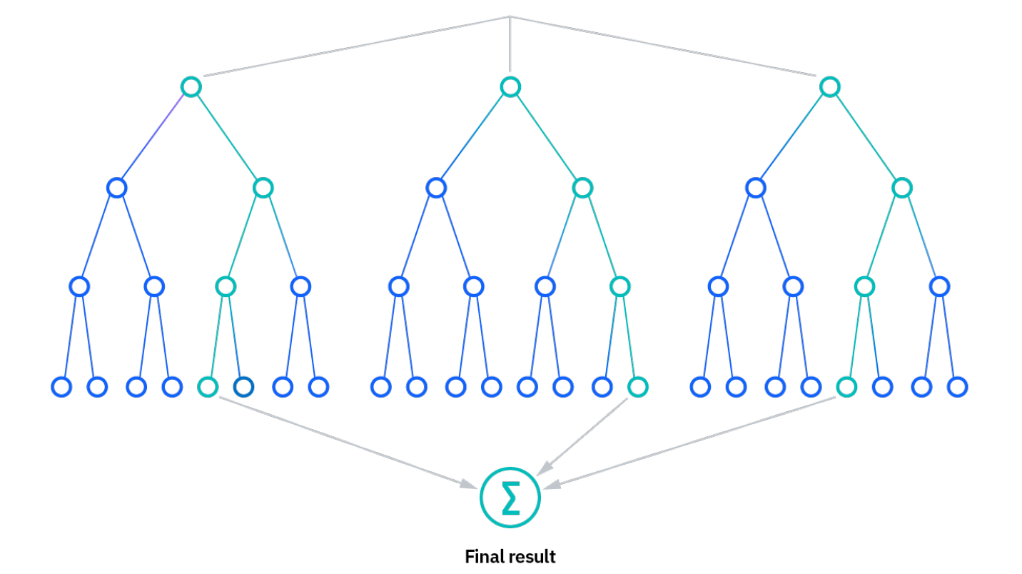
Tip: Here is a short intro to how random forest classification works: https://www.ibm.com/topics/random-forest
//--------------------------------------------------------------
// Run classification (Random Forest)
//--------------------------------------------------------------

// Define prediction bands
// (all Landsat image bands and indices except the QA band)
var predictionBands =  preImage.bandNames().remove('QA_PIXEL');
print('Prediction Bands:', predictionBands)

// Train the classifier with training points only
// "Call" the random forest classifier and train it with the training points
var RFclassifier_y1 = ee.Classifier.smileRandomForest({numberOfTrees:10, seed:100}).train({
  features: training_y1,
  classProperty: 'landcover',
  inputProperties: predictionBands
});
var RFclassifier_y2 = ee.Classifier.smileRandomForest({numberOfTrees:10, seed:100}).train({
  features: training_y2,
  classProperty: 'landcover',
  inputProperties: predictionBands
});

// Print decision trees
var decisionTrees_y1 = RFclassifier_y1.explain();
print('Decision Trees:', decisionTrees_y1);
var decisionTrees_y2 = RFclassifier_y2.explain();
print('Decision Trees:', decisionTrees_y2);

// Classify the median composite
var RFclassification_y1 = preImage
.select(predictionBands)
.classify(RFclassifier_y1);
var RFclassification_y2 = postImage
.select(predictionBands)
.classify(RFclassifier_y2);

// Define visualization parameters
// adjust colors according to your land cover stratification
// define visualization parameters
// 1 = forest; green
// 2 = water; blue
// 3 = urban; red
// 4 = agriculture; light green
// 5 = bare soil; grey
var classVis = {min:1,max:5,palette:['00a661','00a0cd','a40000', 'd5ff6a','d3d2cb']}

// Add classifications to the map
Map.addLayer(RFclassification_y1,classVis,'Year 1 - classification')
Map.addLayer(RFclassification_y2,classVis,'Year 2 - classification')
Display the results, and modify the color palette if needed.
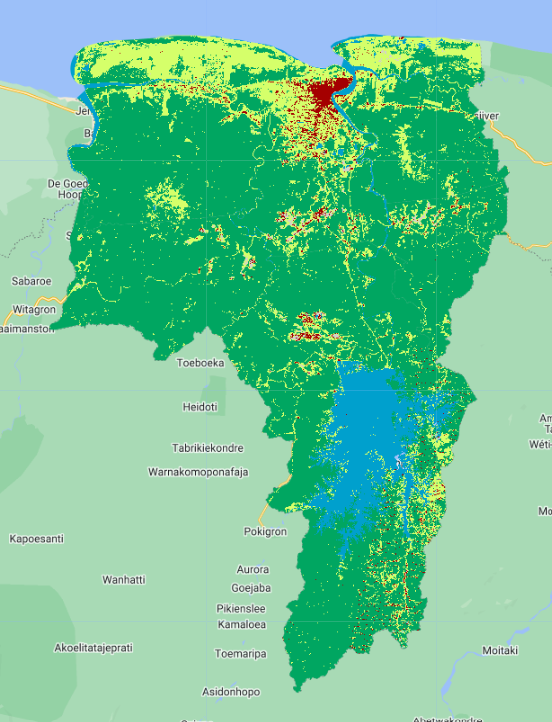
Immediately, we can pick out where some features are mixed up between classes, and where the classifier excels. Which land cover classes seem to have been confused? Do these land cover classes have similar spectral signatures based on our previous graphs?
Run Accuracy Assessment
This is the part in the workflow where you would conduct and accuracy assessment on your two land cover classification maps and go back to refine your input imagery and training data to improve the classification. In the interest of time, we will skip this step for now, but it will be a part of the challenge section.
Tip: Refer to the previous lesson on Mangrove Mapping for an example on how to create an error matrix and calculate accuracy.
Calculate Areas of Change
Now that we have two land cover classification maps for our two different years, we can calculate the areas of various land cover classes in each year see how those areas have changed. We do this using multiply() and sum() to get the area of each pixel with the value of 1 in square meters, sum them all up, and convert them to square kilometers.
Here, we do this process just for our Forest class, but it can be done for all the other classes as well!
//--------------------------------------------------------------
// Calculate class areas
//--------------------------------------------------------------

// Define the pixel category that corresponds to forest
var areaForest_y1 = RFclassification_y1.eq(1).multiply(ee.Image.pixelArea());
var areaForest_y2 = RFclassification_y2.eq(1).multiply(ee.Image.pixelArea());

// Apply reducer to sum areas per pixel
var reducerAreaForest_y1 = areaForest_y1.reduceRegion({
  reducer: ee.Reducer.sum(),
  geometry: aoi,
  scale: 30,
  crs: 'EPSG:4326',
  maxPixels: 1e15
  });
var reducerAreaForest_y2 = areaForest_y2.reduceRegion({
  reducer: ee.Reducer.sum(),
  geometry: aoi,
  scale: 30,
  crs: 'EPSG:4326',
  maxPixels: 1e15
  });

// Convert m^2 to km^2
var areaSqKmForest_y1 = ee.Number(reducerAreaForest_y1.get('classification')).divide(1e6);
print('Forested Area - year 1 (km^2):',areaSqKmForest_y1);
var areaSqKmForest_y2 = ee.Number(reducerAreaForest_y2.get('classification')).divide(1e6);
print('Forested Area - year 2 (km^2):',areaSqKmForest_y2);

Create Change Map
The last step classifying our image into a thematic map consisting of stable and change classes. This can be done rather simply by creating rules or thresholds based on the differences in land cover or index values. In the end, resources, timing, and the patterns of the phenomenon you are trying to map will determine which approach is suitable — or perhaps the activity you are trying to track requires something more advanced, such as a time-series approach that uses more than two dates of imagery.
Here, we create a map showing gains, losses, and stable areas of each land cover type. We do this by writing a function that checks what whether the landcover was forest in both Year 1 and Year 2, and creates a new bands called change in which it labels the pixel as either loss, gain, or stable based on those original landcover values.
Here, we do this process just for our Forest class, but it can be done for all the other classes as well!
//--------------------------------------------------------------
// Create change map
//--------------------------------------------------------------

// Define which class you want to use (let's use forest first)
var landcover = 1;

// Create a function that creates a change map
var classifyChanges = function(image1, image2, landcover) {

    // create an empty image to use as a base for the change map
    var changeImage = ee.Image(0);

    // add a value of 1 to the image where land cover was stable
    changeImage = changeImage.where(image1.eq(landcover).and(image2.eq(landcover)), 1);
    // add a value of 2 to the image where land cover was gained
    changeImage = changeImage.where(image1.neq(landcover).and(image2.eq(landcover)), 2);
    // add a value of 3 to the image where land cover was lost
    changeImage = changeImage.where(image1.eq(landcover).and(image2.neq(landcover)), 3);

    // Return the land cover change image with a single band
    return changeImage.rename('change');
};

// Apply the function to the Year 1 and Year 2 classifictaion maps
//  to get land cover changes between the two
var forestChange = classifyChanges(RFclassification_y1, RFclassification_y2, landcover);

// define visualization parameters
// 1 = stable; light green
// 2 = gain; dark green
// 3 = loss; red
var changeVis = {
    palette: ['e5ffd0','72ad00','c32148'],
    min: 1,
    max: 3 };

// Add change classification to map
Map.addLayer(forestChange.selfMask(),
    changeVis,
    'Forest cover change');

Where was forest gained or lost? Do you think some of these “changes” might just be due to errors in the data prep and classification process?
Calculate Change Areas
Now, using the same process as before, we can calculate the area of each kind of change for each land cover class. What is the difference in the information you can calculate from the land cover maps vs. the change map?
Overall, does net forest area increase/decrease between 2015 and 2022, or does it remain roughly the same? Does this value tell the full story of what is actually going on in the study area? Does gross forest area increase/decrease tell a different story? Are there significant gains and losses that are happening that seem to “balance” each other out when calculating net forest area?
//--------------------------------------------------------------
// Calculate change areas
//--------------------------------------------------------------

// Define the pixel category that corresponds to forest loss and gain
var forestLossArea = forestChange.eq(3).multiply(ee.Image.pixelArea());
var forestGainArea = forestChange.eq(2).multiply(ee.Image.pixelArea());
var forestStableArea = forestChange.eq(1).multiply(ee.Image.pixelArea());

// Apply reducer to sum areas per pixel
var reducerAreaForestLoss = forestLossArea.reduceRegion({
  reducer: ee.Reducer.sum(),
  geometry: aoi,
  scale: 30,
  crs: 'EPSG:4326',
  maxPixels: 1e15
  });
var reducerAreaForestGain = forestGainArea.reduceRegion({
  reducer: ee.Reducer.sum(),
  geometry: aoi,
  scale: 30,
  crs: 'EPSG:4326',
  maxPixels: 1e15
  });
  var reducerAreaForestStable = forestStableArea.reduceRegion({
  reducer: ee.Reducer.sum(),
  geometry: aoi,
  scale: 30,
  crs: 'EPSG:4326',
  maxPixels: 1e15
  });

// Convert m^2 to km^2
var areaSqKmForestLoss = ee.Number(reducerAreaForestLoss.get('change')).divide(1e6);
print('Forest Loss (km^2):',areaSqKmForestLoss);
var areaSqKmForestGain = ee.Number(reducerAreaForestGain.get('change')).divide(1e6);
print('Forest Gain (km^2):',areaSqKmForestGain);
var areaSqKmForestStable = ee.Number(reducerAreaForestStable.get('change')).divide(1e6);
print('Stable Forest (km^2):',areaSqKmForestStable);
Result Reliability
It is important to remember that in such two-date change detection with simple differencing between land cover classifications or spectral indices, many errors are propogated through the process and are inherently present in your final results. For example, there are errors in the satellite data (sensor failures or cloud cover), errors in the preprocessing algorithms (what is done by the data creators (like NASA/ESA) and what is done by you), errors in the sample data (you incorrectly identify forest as agriculture or urban as bare soil), and errors in the classification (misclassifications where spectral differences are similar or training data is poor). It is also very difficult to quantify these errors, and it is hard to know whether they are over- or underestimates of the true values. There are several ways to minimize these errors - or at least statistically quantify their direction and magnitude. One of these is time series change detection, which is covered in the next lesson, and another is sample-based map validation and area estimation, which is partially covered in a later lesson.
Code Checkpoint: https://code.earthengine.google.com/?scriptPath=users%2Febihari%2FSurinameWS%3AChange%20Detection%20-%20Two%20Date%20v3