Processing and cloud masking of composites over Landsat data

Keep the script from Browsing & Preprocessing open, we will continue on.

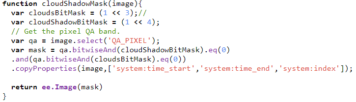
This exercise will demonstrate how to create a cloud-cloud shadow mask using Earth Engine over Landsat imagery. We use the quality assessment (QA) pixel band to create a cloud and shadow mask. Bits 3 and 4 are cloud and cloud shadow, respectively. We define a function which always includes the return command to provide the resultant product.

The QA_PIXEL band is the information channel that characterizes the quality of the pixel regarding cloud and cloud shadow. How to use this info?… If we want to know about a specific function we can go to the ‘Docs’ section and type the function name, then click on the function and see the specification, parameters and application of it. Look closely at the type of object you’re applying to. In this case, we are looking for the bitwiseAnd operator for the object image (ee.Image).

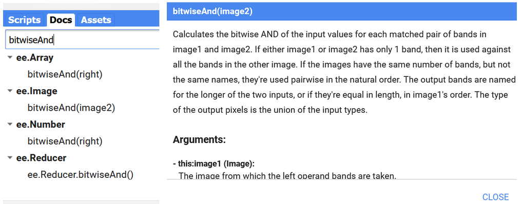
Figure 16. BitwiseAnd function description.

var cloudMask = landsat8_sr.map(cloudShadowMask)
print('cloud_mask: ', cloudMask)


Map.addLayer(cloudMask, {}, 'cloud mask')

// Cloud masking function.
function cloudShadowMask(image) {
  // Bits 3 and 4 are cloud and cloud shadow, respectively.
  var cloudShadowBitMask = (1 << 4);
  var cloudsBitMask = (1 << 3);
  // Get the pixel QA band.
  var qa = image.select('QA_PIXEL');
  // Both flags should be set to zero, indicating clear conditions.
  var mask = qa.bitwiseAnd(cloudShadowBitMask).eq(0)
                .and(qa.bitwiseAnd(cloudsBitMask).eq(0))
                .copyProperties(image,['system:time_start','system:time_end','system:index']);
  return ee.Image(image).updateMask(mask);
}

Through the command .map() we apply the function to the Landsat dataset. We define the visualization parameters: the basic values to be specified are the bands to occupy the blue, green and red channels, plus min and max reflectance value, which will depend on the range of values. Here you have to take in account that Landsat collection 2 values are factored per 10000 by default, with a common max value of 3000. Values higher than 3000 usually fall in the category of cloudy areas, saturated values or outliers derived from radiometric errors of the sensor.

var landsat8_sr_cloud_masked = landsat8_sr.map(cloudShadowMask)
// visualization Landsat 8 collection 2
var visual_lan = {
  bands: ['SR_B4', 'SR_B3', 'SR_B2'],
  min: 0.0,
  max: 0.3,
};

Map.addLayer(landsat8_sr_cloud_masked, visual_lan , 'Cloud masked Landsat')

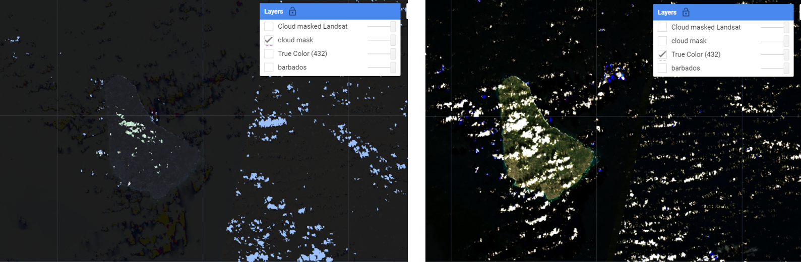
Figure 17. Cloud mask product (left) versus Landsat-8 mosaic (right).

As we see, the black pixels correspond to cloud-free pixels, and the transparent (masked) pixels contain clouds. We can always check the mask structure compared to the true color mosaic and see how well it identified the cloud cover.

Now that the cloud mask has been generated, we apply it to the image collection.

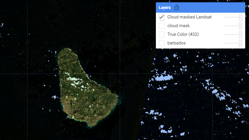
Figure 18. Cloud masked Landsat mosaic.

However we need to compute a value representing the series of SR values. This is called a composite. Usually a statistic as the median works well for composites. Additionally we can clip the image to frame it to the Barbados boundary

var l8_sr_med = landsat8_sr_cloud_masked.median()
.select('SR_B2','SR_B3','SR_B4','SR_B5', 'SR_B6', 'SR_B7')
.clip(barbados_bou)

Map.addLayer(l8_sr_med, visual_lan, 'True Color Landsat Median');

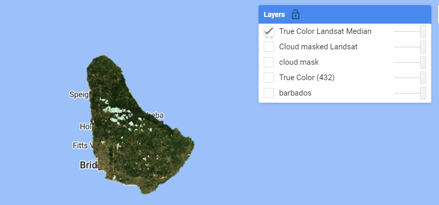
Figure 19. Computed temporal median of a Landsat-8 collection, plus clipped.

We can analyze and compare some very cloudy areas after they have been cloud-masked.

Code Checkpoint: https://code.earthengine.google.com/9c9c29f68ed95883aa41915dd6db87cb.

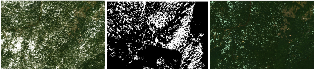
Figure 20. Comparison of products: (left) not masked mosaic, (center) cloud mask, (right) cloud-masked mosaic

Since we see many gaps in the masked image, we can select a longer period in order to have a greater pool of images and higher chance of getting less clouded images.